On learning agent-based models from data

Abstract

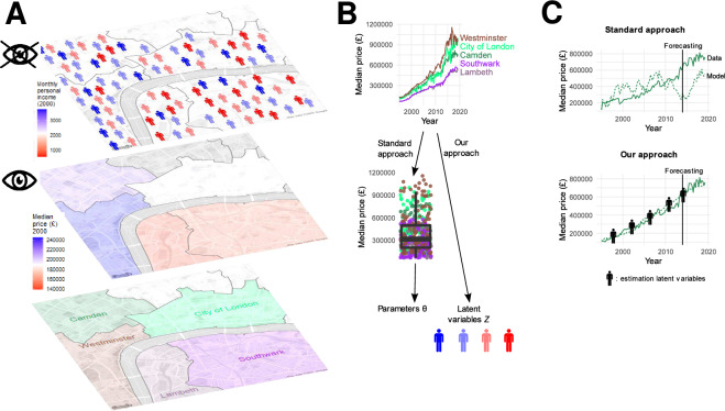
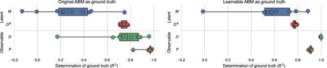
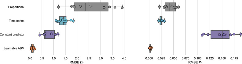
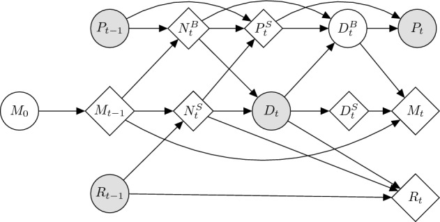
Agent-Based Models (ABMs) are used in several fields to study the evolution of complex systems from micro-level assumptions. However, a significant drawback of ABMs is their inability to estimate agent-specific (or "micro") variables, which hinders their ability to make accurate predictions using micro-level data. In this paper, we propose a protocol to learn the latent micro-variables of an ABM from data. We begin by translating an ABM into a probabilistic model characterized by a computationally tractable likelihood. Next, we use a gradient-based expectation maximization algorithm to maximize the likelihood of the latent variables. We showcase the efficacy of our protocol on an ABM of the housing market, where agents with different incomes bid higher prices to live in high-income neighborhoods. Our protocol produces accurate estimates of the latent variables while preserving the general behavior of the ABM. Moreover, our estimates substantially improve the out-of-sample forecasting capabilities of the ABM compared to simpler heuristics. Our protocol encourages modelers to articulate assumptions, consider the inferential process, and spot potential identification problems, thus making it a useful alternative to black-box data assimilation methods.

Figure 1

Our approach compared to a standard approach towards calibrating an ABM of the housing market. (A) Focusing on the boroughs in the center of London (bottom layer), we consider the yearly average of transaction prices (middle layer) as an example of an observed variable, and the distribution of agent incomes (top layer) as an example of a latent variable. (B) For each borough, we observe a time series of transaction prices. In the standard approach to calibration, modelers could typically calibrate some parameters $\mathrm{\Theta }$ (such as the probability for inhabitants to put their home on sale) by computing the moments of transaction prices across boroughs and years (as represented through a box plot), and minimizing the distance with the same moments in model-generated time series. In our approach, instead, we are able to calibrate the evolution of latent variables Z –in this example, borough-level agent incomes– by exploiting all information contained in time series, rather than reducing this information to specific summary statistics. (C) In the model, prices depend on agent incomes. Thus, since in the standard approach agent incomes are not calibrated, model-generated time series are bound to diverge, even if prices are initialized as in the data. With our approach, as we repeatedly estimate incomes, we can make model-generated time series track empirical ones. This makes it feasible to forecast future prices.

Figure 2

Quality of estimation in synthetic experiments with traces generated by the original (left) and learnable (right) ABM. For each variable, we report the coefficient of determination $R^2$ between the original values and the estimates for each trace. We represent each trace as a dot, with whisker plot as a summary for each variable. Whiskers extend from the minimum to the maximum value, while boxes range from the 25th to the 75th percentile.

Figure 3

Estimates for $M_{t,x,k}$, $D_{t,x,k}^B$, $P_{t,x}$, $D_{t,x}$ compared to the traces generated with the original ABM, in a single experiment, chosen as the median experiment in terms of estimation quality.

Figure 4

Out-of-sample forecasting error for our method compared to alternative benchmarks for the number of transactions $D_t$ (left) and prices $P_t$ (right). We show the forecasting error as the RMSE of each time series. We consider the same 10 traces as in the experiments above, and show results for each of the 10 traces as a dot and a whisker plot as a summary. Whiskers extend from the minimum to the maximum value, while boxes range from the 25th to the 75th percentile.

Figure 5

Graphical model diagram of the learnable ABM for a time step t. See Materials & Methods “Model description” section for notation. Diamonds indicate deterministic variables, white circles indicate latent stochastic variables, grey circles indicate observed stochastic variables.

References

1. Wilensky, U. & Rand, W. An Introduction to Agent-Based Modeling: Modeling Natural, Social, and Engineered Complex Systems with NetLogo (Mit Press, 2015).
1. Railsback, S. F. & Grimm, V. Agent-Based and Individual-Based Modeling: A Practical Introduction. (Princeton University Press, 2019).
1. Axelrod R. The dissemination of culture: A model with local convergence and global polarization. J. Confl. Resol. 1997;41(2):203–226. doi: 10.1177/0022002797041002001. - DOI
1. Lux T. Estimation of agent-based models using sequential monte Carlo methods. J. Econ. Dyn. Control. 2018;91:391–408. doi: 10.1016/j.jedc.2018.01.021. - DOI
1. Delli Gatti D, Grazzini J. Rising to the challenge: Bayesian estimation and forecasting techniques for macroeconomic agent based models. J. Econ. Behav. Organ. 2020;178:875–902. doi: 10.1016/j.jebo.2020.07.023. - DOI