Hydration solids

Abstract

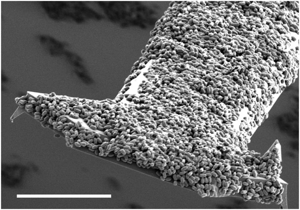
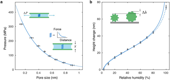
Hygroscopic biological matter in plants, fungi and bacteria make up a large fraction of Earth's biomass¹. Although metabolically inert, these water-responsive materials exchange water with the environment and actuate movement^2-5 and have inspired technological uses^6,7. Despite the variety in chemical composition, hygroscopic biological materials across multiple kingdoms of life exhibit similar mechanical behaviours including changes in size and stiffness with relative humidity^8-13. Here we report atomic force microscopy measurements on the hygroscopic spores^14,15 of a common soil bacterium and develop a theory that captures the observed equilibrium, non-equilibrium and water-responsive mechanical behaviours, finding that these are controlled by the hydration force^16-18. Our theory based on the hydration force explains an extreme slowdown of water transport and successfully predicts a strong nonlinear elasticity and a transition in mechanical properties that differs from glassy and poroelastic behaviours. These results indicate that water not only endows biological matter with fluidity but also can-through the hydration force-control macroscopic properties and give rise to a 'hydration solid' with unusual properties. A large fraction of biological matter could belong to this distinct class of solid matter.

Extended Data Figure 1:. Spore-coated cantilever.

Scanning electron microscopy image of a spore-coated cantilever. Scale bar ~20 μm. The cantilever is T-shaped, and it is approximately 300 μm long and 30 μm wide, except near the free end where the width is approximately 60 μm.

Extended Data Figure 2:. Cantilever deflection signals.

Representative cantilever deflection signals following photothermal pulses shown for a range of relative humidity levels. Deflection signals are normalized so that peak-to-peak deflection corresponds to 1. All curves are obtained with the same spore-coated cantilever. They are representative of curves from all five cantilevers used in Fig. 1d.

Extended Data Figure 3:. Microstructure and properties of spores.

a, Scanning electron microscopy image of the spores of B. subtilis. Scale bar: 500 nm. Wild type spores of B. subtilis are approximately 650 nm in diameter and 1 um to 1.5 um in length. b, Illustration of the cross section of spores of B. subtilis showing the cortex and coat layers that surround the core, which contains the genetic material. The coat is a proteinaceous, water-permeable layer. AFM images of the outer surface of the coat reveals an assembly of parallel rodlets formed by coat proteins with ~ 8 nm periodicity. The cortex, also a water permeable layer, is a loosely crosslinked network of peptidoglycan that is similar in structure to that of vegetative cells. The vegetative peptidoglycan in B. subtilis has an average diameter of 4 nm, as observed in AFM images. The thicknesses of the coat and the cortex layers are approximately 70 nm each (see Methods). The spore core contains proteins and DNA. The core is dehydrated and the DNA is packed in a crystalline state. Elastic modulus measurements of DNA films in crystalline state show the Young’s modulus of these films to be approximately 1.1 GPa, suggesting that the core is a stiff solid rather than a fluid. This assumption is also supported by the observation that soluble biomolecules are immobile in the dehydrated cores of dormant spores but gain mobility upon germination when the core gets hydrated. The spore water, however, exhibits rotational mobility, as indicated by the observations of short rotational correlation times of D₂O in spores. This observation also indicates that water in spores is not in an ice-like (solid) state.

Extended Data Figure 4:. Relative effect of the photothermal pulse.

Shifts in the resonance frequency of spore-coated cantilevers are sensitive to the amount of water exchange. We used this effect to compare relative effects of the photothermal pulse and RH. Here we plot the relative changes in fundamental resonance frequency of a cantilever coated with spores in two cases: (left, red bar) as a result of photothermal pulse and (right, purple bar) in response to a change in relative humidity from 80% to 10%. The results are given as percentages. They indicate that the perturbation due to the photothermal pulse is small, and therefore, the transient deflections of the cantilever in response to photothermal pulses reflect approximately the state of the spore at the set-point level of the relative humidity.

Extended Data Figure 5:. Time constants and the total spore mass.

The spore quantities are represented by spore mass estimated from the shifts in cantilever resonance frequencies. Time constants are plotted for wild type (square) and B. subtilis cotE gerE (circle) spores. According to the data, there is a lack of clear association between the time constant and the total spore mass, however the effect of spore type results in a statistically significant change in time constants: Mean time constant at 50% RH for Wild type [square] is ~118 ms and ~47.1 ms for B. subtilis cotE gerE [circle] (one-tailed T, p<.01).

Figure 1:. Slow water transport in spores.

a, Change in spore height versus RH. Data are mean ±s.e.m. (n=20). b, Spores deposited on a cantilever are perturbed by weak photothermal pulses. c, Spores are subjected to different set point RH values to vary the pore sizes. Blue areas represent pore water and green areas represent pore walls. The curves are examples of experimental data showing the cantilever deflection response to the photothermal stimulus (yellow region). The relaxation curves following the pulse (dark blue) are used to determine time constants. d, Time constants plotted against set point RH. Data are mean ± s.e.m. (n = 5 measurements with separate cantilevers). e, Inverse time constants (d) plotted against pore diameter. Solid blue line: Least squares fit to data with a power-law relationship having an exponent equal to 1.9. The data point at 10% RH is excluded from the fit as the time constant is close to the pulse duration. Data are mean ± s.e.m. (n = 5 measurements with separate cantilevers). f, Activation energy ($E_a$) versus RH. Data points are individual measurements. Repeated measurements done with three cantilevers are represented with marker shapes (circle, square, and diamond).

Figure 2:. The hygroelastic model.

a, Schematic of the hydration force (grey) and its exponentially-decaying smooth component (blue). Distance values are given to indicate the short, sub-nanometer range of the hydration forces. b, Hydration forces between pore walls act as a nonlinear spring. This spring dominates all other mechanical restoration forces, including the stiffness of the biomolecular matrix forming the pores. Forces due to dehydration (decrease in the chemical potential of water at low RH) act effectively as a decrease in pore fluid pressure ($\Delta P$), acting on the nonlinear spring and compress the pores, which is similar to the effect of mechanical stresses ($\Delta c$). c, Illustration of energy barriers against changes in pore size due to changing RH or external forces. d, The hygroelastic model predicts that the pore water will exhibit solid-like characteristics when perturbed at short timescales (faster changes), illustrated here with an AFM tip applying an oscillating force.

Figure 3:. Dominant role of hydration forces.

a, The magnitude of the effective pressure due to chemical potential of water, calculated from RH, temperature, and the molar volume of water, plotted against pore size (diamonds). Data are mean ±s.e.m. (n=20). Solid line is an exponential fit to the data. Dashed lines are extrapolations. Illustrations show the balance between the chemical potential, $\Delta P$, and the force due to a nonlinear spring, which determines the pore size, denoted by $x$. b, Predicted spore height change with RH according to Eq. (2), solid blue) plotted with the mean height change against RH (diamonds). Data are mean ±s.e.m. (n=20 for RH from 10% to 80%, and n = 19 for RH = 3% and 100%). Dashed blue line corresponds to Eq. (2) after the substitution $\varrho \to 0.96\varrho$ to account for background forces.

Figure 4:. Strong nonlinear elasticity.

a, Theoretical stress-strain curves for different values of $l$. b, A representative experimental force-indentation curve using a spherical AFM tip. The horizontal bar under the AFM tip illustrates the contact diameter (2a). c, Contact stiffness versus indentation depth (green dotted line) and the theoretical contact stiffness of a linear elastic material with matching peak contact stiffness (solid black line). d-f, Force-indentation curves on multiple spores (green dotted lines) from B. subtilis (d), B. subtilis cotE gerE (e), and B. thuringiensis (f). Solid grey curves: least squares fits based on Eq. (5). g, Values of $l$ determined in (d-f). Data points from each individual spore are grouped vertically. The width of the 95% confidence intervals determined by the fit were less than 8% of the respective value of $l$ for 59 of 63 curves, and between 15% and 21% for the remaining 4 curves. Horizontal line: $l$ estimated independently using the change in spore height with RH. h,i, Stress-strain and tangent modulus-strain curves based on Eqs. (3,4) using the mean values of $l$ in (g), plotted to highlight the degree of nonlinearity.

Figure 5:. The hygroelastic transition.

a, AFM force-distance curves are recorded at different modulation rates of vertical position. In the diagrams on the right, dashed lines represent the time-dependent tip position and the solid lines represent the corresponding force. Contact time is indicated with a left-right arrow. b, Examples of force-distance curves recorded with slow (1 Hz) and fast (2 kHz) modulation rates. c, Elastic modulus estimated from force-distance curves plotted against the contact time. Color represents individual spores and marker shape represents the AFM method used: Force ramp (round), Peak Force Tapping at 125 Hz (square) and at 2 kHz (diamond). d, Schematic of the standard linear solid model. $E_s$ and $E_f$ are elastic moduli, $\eta$ is the viscosity. e, f, Frequency response (e) and the loss tangent of the model in (d). Frequency is normalized to $E_s∕\eta$. g, Normalized step response of the model in (d) for a step change in displacement (grey) and a step change in force (blue). Time is normalized to $\eta ∕E_s$. $E_l$, $E_h$ are defined in (e), and they correspond to long-term and short-term elastic moduli.

References

1. Bar-On YM, Phillips R & Milo R The biomass distribution on Earth. Proceedings of the National Academy of Sciences 115, 6506–6511 (2018). 10.1073/pnas.1711842115 - DOI - PMC - PubMed
1. Dawson C, Vincent JFV & Rocca A-M How pine cones open. Nature 390, 668–668 (1997). 10.1038/37745 - DOI
1. Elbaum R, Zaltzman L, Burgert I & Fratzl P The Role of Wheat Awns in the Seed Dispersal Unit. Science 316, 884–886 (2007). 10.1126/science.1140097 - DOI - PubMed
1. Fratzl P & Barth FG Biomaterial systems for mechanosensing and actuation. Nature 462, 442–448 (2009). 10.1038/nature08603 - DOI - PubMed
1. Dumais J & Forterre Y “Vegetable Dynamicks”: The Role of Water in Plant Movements. Annual Review of Fluid Mechanics 44, 453–478 (2012). 10.1146/annurev-fluid-120710-101200 - DOI
Publication types