Generalized precursor prediction boosts identification rates and accuracy in mass spectrometry based proteomics

Abstract

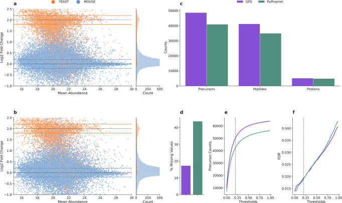
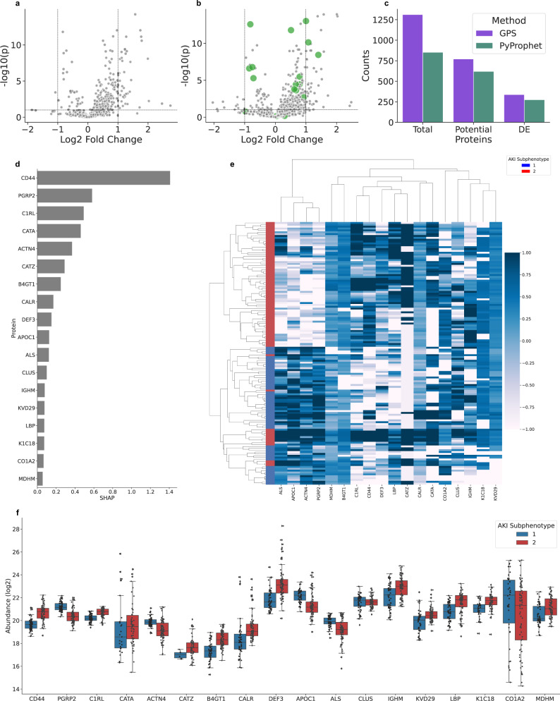
Data independent acquisition mass spectrometry (DIA-MS) has recently emerged as an important method for the identification of blood-based biomarkers. However, the large search space required to identify novel biomarkers from the plasma proteome can introduce a high rate of false positives that compromise the accuracy of false discovery rates (FDR) using existing validation methods. We developed a generalized precursor scoring (GPS) method trained on 2.75 million precursors that can confidently control FDR while increasing the number of identified proteins in DIA-MS independent of the search space. We demonstrate how GPS can generalize to new data, increase protein identification rates, and increase the overall quantitative accuracy. Finally, we apply GPS to the identification of blood-based biomarkers and identify a panel of proteins that are highly accurate in discriminating between subphenotypes of septic acute kidney injury from undepleted plasma to showcase the utility of GPS in discovery DIA-MS proteomics.

Fig. 1. Overview figure depicting GPS and the methods and data used for evaluation.

GPS is first visualized in (a) and split into two groups. The first part of (a) visualizes the training procedure for the GPS models. The data from Yeast samples were first acquired at different gradient lengths from two different mass spectrometers and totaled 3.75 million precursors from 128 sample files. This data was then split into a train and test set. The training set was further filtered using a k-fold (k = 10) self-denoising algorithm where an ensemble of logistic regression models are trained for each fold and vote on the held-out data to determine the set of true precursors. This removal of false precursors results in a filtered training set of 2.8 million precursors. Two models, one SVM and one XGBoost, were then trained on the filtered and unfiltered training data for a total of four models. These trained models are then applied to new data to predict and score precursors to validate extracted signal in a DIA-MS experiment. b Visualizes the 4 separate methods used to validate GPS and compare it to existing methods, along with the data that are used for each analysis. To directly evaluate how GPS generalizes to new data, we measured the performance of the four classifiers on the yeast data, mouse-kidney data, and a subset of the human plasma data. We then measured and compared the identification rates of GPS and PyProphet using the mouse-kidney data in an entrapment FDR analysis. We then evaluated the quantitative accuracy of the validated identifications of GPS compared to PyProphet by analyzing a set of two-species mixture samples consisting of two groups and comparing the number of identifications that fall within the expected ratios. Created with BioRender.com.

Fig. 2. Generalization of GPS to three distinctly different sample types.

As a first analysis, we directly evaluated the ability of GPS to generalize to new data. a–c Show the average number of precursors identified with the four GPS models (GPS XGB Filter, GPS XGB No Filter, GPS SVM Filter, GPS SVM No Filter) and two PyProphet models (Pyprophet XGB and PyProphet LDA). The dotted red lines represent a 1% FDR cutoff so the performance of each tool on each of the three datasets can be visualized at the specific cutoff. The error bands are based on the 95% confidence intervals calculated at each FDR cutoff. a Displays the number of precursors identified on the yeast data, which represents the most simple of the three tested sample types for generalization and the number of proteins is lower, and the number of precursors in the sample directly match the spectral library used. b Displays the number of identified precursors for the mouse-kidney data, which represents a more complex proteome. Here, PyProphet does not perform as well as the yeast data, which it was trained on, suggesting that GPS generalizes to new data more effectively. c Displays the number of identified precursors at different thresholds for a subset of human plasma samples. These samples were searched using a human tissue library and represent a large search space scenario where the number of precursors does not match the precursors in the spectral library. Here, GPS provides the most identifications at a 1.0% FDR showing how effectively it can generalize independent of the search space. d Contains box plots indicating the measured precision for each model at classifying only true targets. The colors of each bar represent the three different datasets. The colors of the horizontal dotted lines correspond to the indicated models in (a–c) and are placed at the mean precision for each model across all three datasets. The GPS XGB Filter model had the highest measured average precision across all three sample types. GPS SVM Filter had a comparable measured average precision, indicating the importance of filtering the training data to maximize precision in a precursor classifier.

Fig. 3. Entrapment FDR analysis and precursor identification benchmark.

This figure displays the ability of GPS to eliminate false precursors (Yeast precursors) from analysis using highly precise precursor prediction. On a first pass, precursors are predicted to remove false target precursors from FDR analysis. The precursors that are predicted as true targets are re-extracted to adapt the search space and ensure that only true targets are considered during distribution modeling and FDR calculation. a, b Display score distributions calculated by GPS for all extracted precursors in the mouse samples using a mouse-yeast species mixture spectral library. a Displays the unfiltered score distributions from GPS for Mouse precursors in the library in orange, Yeast precursors in the library as blue, and Decoys in the library as green. A large peak in the bimodal target distribution can be visualized as overlapping with the yeast distribution and decoy distribution. b Displays a filtered score distribution after peak group predictions using GPS and the removal of false targets from consideration. Here we can see that the yeast precursor peak is almost completely eliminated from contention, and the bimodality of the false target (orange target distribution) is lessoned in the region overlapping with the decoy distribution. These two panels display how GPS can control the search space so that the FDR can be controlled in a stable manner. c Displays the number of true mouse target precursor counts at increasing FDR thresholds for GPS and PyProphet. The dotted red line indicates a 1% FDR to visualize the performance at that cutoff. The error bands are based on the 95% confidence intervals calculated at each FDR cutoff. At all cutoffs GPS identifies more precursors than PyProphet. d Displays the Yeast FDR rates, defined as the number of Yeast identifications divided by the total number of identifications, at increasing FDR thresholds. The red dotted line indicates a 1% FDR and the dotted black line represents y = x, where the Yeast FDR should correspond directly to the measured FDR. The error bands are based on the 95% confidence intervals calculated at each FDR cutoff. The measured Yeast FDR is lower using GPS at all thresholds compared to PyProphet, and is more strict at higher thresholds than PyProphet while still identifying more precursors at the same thresholds.

Fig. 4. Quantification accuracy of GPS evaluated by a two-species mixture spike-in dataset.

We evaluated the quantification accuracy of GPS by analyzing a two-species mixture of yeast peptides spiked-in into a constant mouse-kidney proteome background with two groups of ten technical replicates each. Each group of samples contained the same concentration of Mouse-Kidney proteins, while one group contained 4× more yeast peptides and we measured the number of precursors that mapped correctly into the expected ratio of their species (0.0 ± 0.2 log2 fold change for Mouse precursors and 2.0 ± 0.2 log2 fold change for Yeast precursors. a displays the mean abundance of precursors identified using GPS against their log2 fold change and colored by their mapped species. Histogram plots directly to the right of these scatter plots display the distribution of the species mixture on the log2 fold change scale. The expected ratio regions are highlighted to display which precursors were considered as ratio-validated. b displays the same as (a) but for PyProphet. c Displays the overall counts of ratio-validated precursors, peptides, and proteins, from the regions highlighted in (a, b) for GPS and PyProphet. From these validated regions, GPS identifies more precursors, peptides, and proteins than PyProphet. d Shows the percentage of missingness in the quantitative matrices for GPS and PyProphet. Here, GPS decreased the number of missing values by 60.51% compared to PyProphet. This is important in context with (c), as GPS is able to provide a greater number of accurately quantified precursors and a substantially more complete data matrix as measured by the % missing values. In order to provide an evaluation beyond the ratio-validated cutoff, we measured the number of identified precursors and the FDR at increasing log2 fold change thresholds from the expected ratios of the species mixture in (e, f). e Displays the number of precursors identified and quantified at increasing thresholds from the expected values. GPS identifies more precursors at every threshold compared to PyProphet. f Displays the the FDR as a function of increasing thresholds from the expected ratios of each proteome in the mixture. Here, we can see at low thresholds, GPS displays a slightly higher FDR, but the two tools even out over the measured thresholds, with GPS having a lower FDR further away from the expected ratios. GPS is able to identify more precursors while maintaining a comparable FDR to PyProphet over the increasing thresholds measured. The dotted horizontal lines visualize the number of precursors and measured FDR at the ±0.2 thresholds used for ratio-validated quantification.

Fig. 5. The application of GPS for the identification of blood-based biomarkers in septic AKI.

The analysis performed in this application serves two main purposes. One, to evaluate GPS in a large search space and compare the number of potentially comparable proteins to PyProphet. Two, to apply GPS to identify a group of biomarkers using machine learning with recursive feature elimination and explainable artificial intelligence (RFE-SHAP) that could be useful in stratifying subphenotypes of septic AKI (total n = 141, less severe (n = 60), and more severe (n = 80)). a Displays a Volcano plot for differentially abundant proteins identified using PyProphet. b Displays a Volcano plot for differentially abundant proteins identified using GPS with the 18 proteins selected as potential biomarkers highlighted in green. c Displays the overall counts of the total proteins identified by each method (GPS and PyProphet), the potential proteins (proteins found in minimum ten replicates per group), and the statistically significant differentially abundant proteins (corrected P value < 0.1). At all levels, GPS identified more proteins than PyProphet for the measured data. To identify a group of proteins that could be important in differentiating between subphenotypes of septic AKI, we employed machine learning and RFE-SHAP to pick the optimal set of proteins used for classification. d Displays the 18 proteins selected using RFE-SHAP analysis and their mean importance calculated by SHAP in predicting AKI subphenotypes. CD14 was found as largely the most important protein, with many other documented infection and inflammation markers included in the list. e Shows a clustermap of the AKI samples using the 18 selected proteins. Colored by subphenotype on the y-axis, it is clear that the selected proteins are accurate in stratifying the defined AKI subphenotypes. f Visuzlies the box and swarm plots for the abundance of the 18 selected proteins grouped by AKI subphenotype. The boxes represent the interquartile range of the protein abundances with the swarm plot showing the individual measurements.

References

1. Gessulat S, et al. Prosit: proteome-wide prediction of peptide tandem mass spectra by deep learning. Nat. Methods. 2019;16:509–518. doi: 10.1038/s41592-019-0426-7. - DOI - PubMed
1. Yang Y, et al. In silico spectral libraries by deep learning facilitate data-independent acquisition proteomics. Nat. Commun. 2020;11:1–11. - PMC - PubMed
1. Tiwary S, et al. High-quality MS/MS spectrum prediction for data-dependent and data-independent acquisition data analysis. Nat. Methods. 2019;16:519–525. doi: 10.1038/s41592-019-0427-6. - DOI - PubMed
1. Zhou XX, et al. PDeep: predicting MS/MS spectra of peptides with deep learning. Anal. Chem. 2017;89:12690–12697. doi: 10.1021/acs.analchem.7b02566. - DOI - PubMed
1. Rosenberger G, et al. A repository of assays to quantify 10,000 human proteins by SWATH-MS. Sci. Data. 2014;1:1–15. doi: 10.1038/sdata.2014.31. - DOI - PMC - PubMed
Publication types