Processing macromolecular diffuse scattering data

Abstract

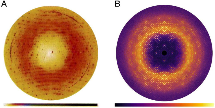
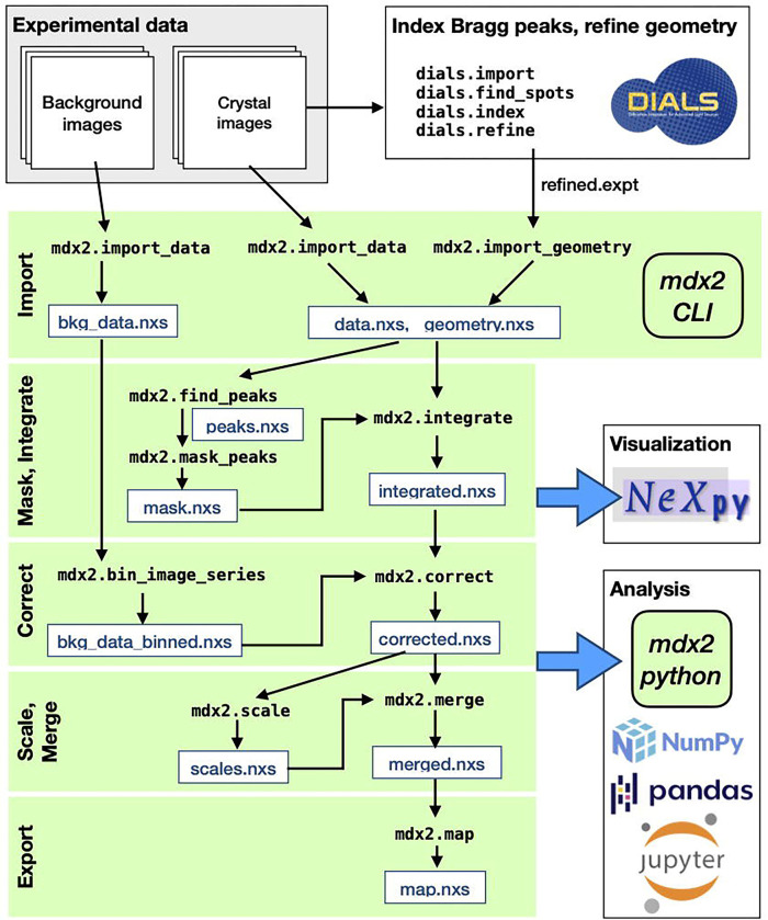
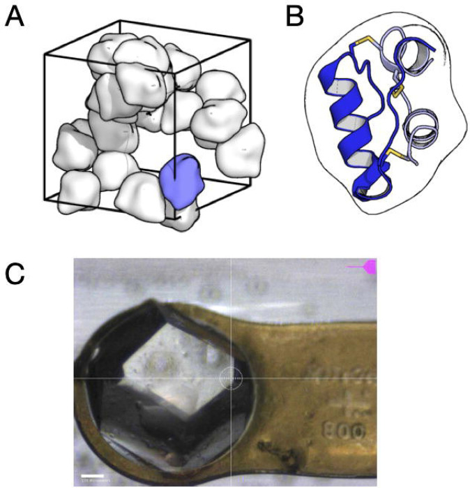
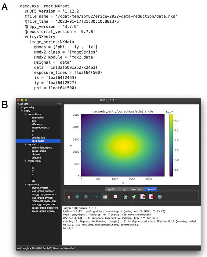
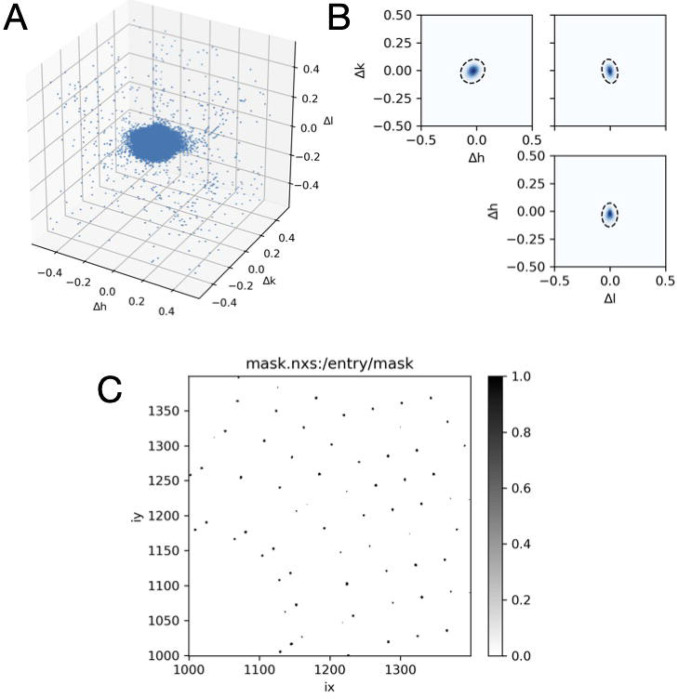
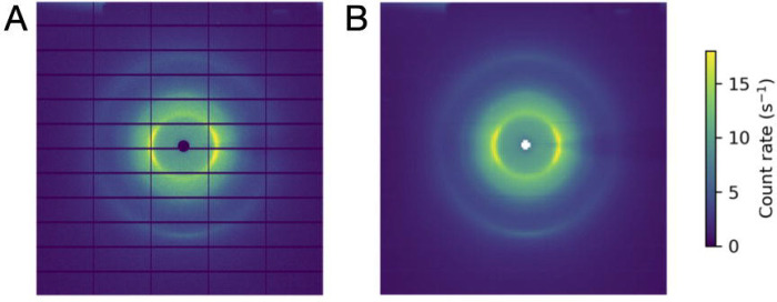
Diffuse scattering is a powerful technique to study disorder and dynamics of macromolecules at atomic resolution. Although diffuse scattering is always present in diffraction images from macromolecular crystals, the signal is weak compared with Bragg peaks and background, making it a challenge to visualize and measure accurately. Recently, this challenge has been addressed using the reciprocal space mapping technique, which leverages ideal properties of modern X-ray detectors to reconstruct the complete three-dimensional volume of continuous diffraction from diffraction images of a crystal (or crystals) in many different orientations. This chapter will review recent progress in reciprocal space mapping with a particular focus on the strategy implemented in the mdx-lib and mdx2 software packages. The chapter concludes with an introductory data processing tutorial using Python packages DIALS, NeXpy , and mdx2 .

Figure 1.

Reciprocal space maps of cubic insulin. (A) A diffraction image recorded on X-ray film, digitized, and processed to remove background and polarization effects. A cloudy pattern and halos surrounding the Bragg peaks are superimposed on the largely isotropic diffuse scattering. Ring features are background scattering from the aluminum windows. Reproduced with permission from (Caspar et al., 1988). (B) Central section (hk0) through the diffuse scattering map reconstructed using mdx2 from fine-sliced rotation data collected using a photon-counting detector (see tutorial in Section 3).

Figure 2.

Workflow for reciprocal space reconstruction using mdx2. Rotation data from crystals and corresponding background images are collected using procedures described in Chapter 1 (Pei et al., 2023). Bragg peaks in the crystal images are processed using DIALS in order to refine the diffraction geometry. Using the mdx2 command-line interface (CLI), the DIALS geometry and diffraction data are imported in NeXus-formatted hdf5 files (.nxs extension) for convenient visualization using NeXpy. Subsequent mdx2 CLI programs (green shading) integrate, correct, scale, and merge the data to produce a three dimensional reciprocal space map (see tutorial in Section 3). At each stage of processing, analysis is performed in Python using mdx2 together with standard scientific packages (see Section 3.7).

Figure 3.

Geometry of reciprocal space reconstruction. (A) An X-ray beam (magenta arrow) is incident on a crystal (cyan) and scattering is recorded on a two-dimensional detector (blue rectangle). Each detector pixel is projected onto the surface of the Ewald sphere, drawn centered on the crystal. The projection (yellow points) is illustrated for a particular scattering direction (green arrow). (B) The same geometry as (A) viewed in the plane formed by the incident and scattered wavevectors (${\mathbf{s}}_0$ and ${\mathbf{s}}_1$). In the Ewald construction, the origin of reciprocal space $\left(\mathbf{O}\right)$ is placed as shown so that the scattering vector $\mathbf{s}$ lies on the surface of the sphere. The blue pattern represents a slice through the reciprocal space intensity $I\left(\mathbf{s}\right)$ with lightly shaded clouds representing diffuse scattering and darker circles representing Bragg peaks at the reciprocal lattice points. (C) The pattern of scattering depends on the intersection of $I\left(\mathbf{s}\right)$ with the Ewald sphere (orange region), which rotates as the crystal rotates. (D) Scattering data recorded at different orientations (slices are drawn with finite thickness to illustrate continuous rotation during exposure) are merged in three dimensions to recover the reciprocal space map (first set of arrows), and known symmetries may be used to further complete the reconstruction (bottom arrow).

Figure 4.

Scaling model for a triclinic lysozyme dataset from refinement using mdx-lib. Panels are arranged with rows corresponding to the eleven sweeps of data distributed over four crystals (see original publication for details) and columns corresponding to the four terms in the scaling model in Equation 21 (left to right): $c,b,a$, and $d$. Reproduced under CC-BY-4.0 license from (Meisburger et al., 2020).

Figure 5.

Insulin crystal that produced the dataset used in the tutorial. (A) Insulin from Bos taurus was crystallized using a Zn-free condition in the space group I2₁3. The unit cell (wireframe box) contains 24 copies of the asymmetric unit (smooth molecular surfaces). The packing arrangement has large channels occupied by disordered solvent. (B) The asymmetric unit, drawn in the same orientation as the blue blob in (A), contains a single insulin molecule consisting of two alpha-helical chains (blue and gray cartoons) cross-linked by three disulfide bonds (yellow sticks). (C) Image taken during data collection of the ~800 micron crystal mounted on a Kapton loop and held within a plastic capillary to maintain hydration. The datset processed in this tutorial consists of a single 50-degree sweep (0.1 degrees and 0.1 seconds per frame). Because of the large crystal size and high symmetry, a single sweep is sufficient for a complete reciprocal space map.

Figure 6.

Plots from the DIALS report that illustrate a successful geometry refinement. The scan-varying model allows for the unit cell constants (A) and setting angles (B) to vary smoothly throughout the scan. Refinement minimizes the difference between observed and predicted coordinates of the Bragg peaks on the detector surface (C) and image number $Z$ in the scan (D). The parameter changes are minimal during the scan, and the errors are much less than one pixel or image. Furthermore, there are no sudden jumps or outliers in panel (D), which might indicate that the crystal had slipped or cracked during data collection.

Figure 7.

NeXus files produced by mdx2 and visualization using NeXpy. (A) The file data.nxs contains the raw diffraction data as a 3-dimensional array with associated metadata in an NXdata object. The text representation of the file was produced by the function mdx2.tree. (B) The more complex file geometry.nxs has many NeXus objects organized in a hierarchical fashion (tree view, left panel). Objects can be plotted by double-clicking (here, the solid_angle correction mapped over the detector surface). Axes are generated automatically from the metadata.

Figure 8.

Rocking curve showing Bragg diffraction and diffuse scattering. An intense peak was selected that passed slowly through the Ewald sphere (lying close the rotation axis in reciprocal space). (A) The Bragg peak in frame 42 where it’s intensity is maximum. The intensity decays quickly to background over several pixels (note the logarithmic color scale; pixels with zero counts are colored gray). (B) The total number of counts within the region around the Bragg peak in (A) as a function of rotation angle. The central bell-shaped peak is the Bragg diffraction, and the gradual tails are diffuse halos (arrows). The plots were generated using built-in functions of the nexusformat package (see Section 3.2).

Figure 9.

Bragg peaking masking. (A) Strong pixels (those exceeding a count threshold) are mapped into reciprocal space and plotted as a function of distance from the nearest Bragg peak (axes are fractional Miller indices). (B) The points are fit to a three-dimensional Gaussian probability distribution, here shown as a dashed contour line at 3 standard deviations superimposed on orthogonal projections of the distribution in (A). The Gaussian fit accouts for potential anisotropy due to crystal properties and errors in the model of diffraction geometry. (C) A mask is generated for all pixels in each image according to the Gaussian fit.

Figure 10.

Image processing for background subtraction. (A) An example background image (1 degree oscillation, 1 second exposure) from the insulin rotation dataset. (B) The same image after binning to improve signal-to-noise. Background corrections are computed for each voxel in the reciprocal space map by interpolation of the binned image stack.

Figure 11.

Scale factor per image in a rotation set after refinement using mdx2.

Figure 12.

Slice through the reciprocal space map of insulin visualized using NeXpy.

Figure 13.

Intensity statistics for the insulin diffuse scattering dataset after scaling. (A) The mean (blue) and standard deviation (orange) of intensity were computed within each resolution shell for the merged reciprocpal space map. The variations in the diffuse pattern are much smaller than the isotropic component. However, they are larger than the noise in the data (average measurement error, propagated from Poisson statistics), shown in green. (B) The dataset was split into equivalent halves and merged separately, and the Pearson correlation was computed between these half datasets as a function of resolution (1/s). By this measure, the variations in the diffuse pattern contain signficant signal up to ~2 Å resolution. The dip at low resolution is related to the strength of the halo features relative to the background in this dataset.

References

1. Ayyer K., Yefanov O. M., Oberthür D., Roy-Chowdhury S., Galli L., Mariani V., Basu S., Coe J., Conrad C. E., Fromme R., & others. (2016). Macromolecular diffractive imaging using imperfect crystals. Nature, 530(7589), 202–206. - PMC - PubMed
1. Busing W. R., & Levy H. A. (1967). Angle calculations for 3- and 4-circle X-ray and neutron diffractometers. Acta Crystallographica, 22(4), 457–464. 10.1107/S0365110X67000970 - DOI
1. Caspar D., Clarage J., Salunke D., & Clarage M. (1988). Liquid-like movements in crystalline insulin. Nature, 332(6165), 659–662. - PubMed
1. Chapman H. N., Fromme P., Barty A., White T. A., Kirian R. A., Aquila A., Hunter M. S., Schulz J., DePonte D. P., Weierstall U., & others. (2011). Femtosecond x-ray protein nanocrystallography. Nature, 470(7332), 73–77. - PMC - PubMed
1. Clarage J. B., & Phillips G. N. Jr (1997). [21] analysis of diffuse scattering and relation to molecular motion. In Methods in enzymology (Vol. 277, pp. 407–432). Elsevier. - PubMed
Publication types