A non-oscillatory, millisecond-scale embedding of brain state provides insight into behavior

Abstract

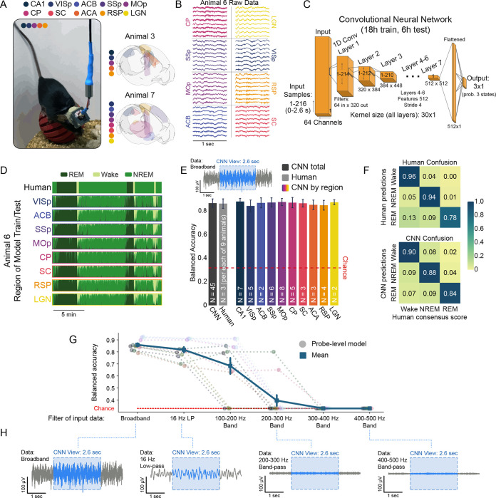
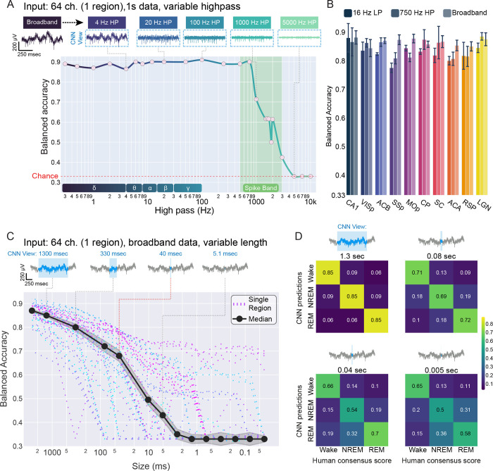
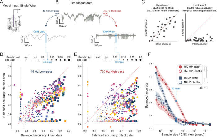
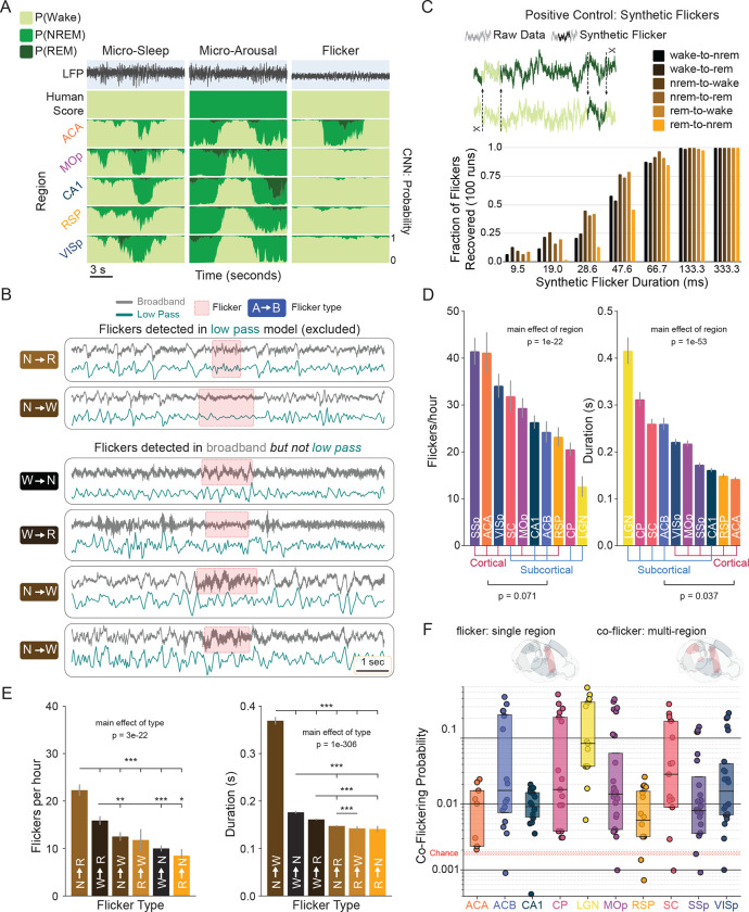
Sleep and wake are understood to be slow, long-lasting processes that span the entire brain. Brain states correlate with many neurophysiological changes, yet the most robust and reliable signature of state is enriched in rhythms between 0.1 and 20 Hz. The possibility that the fundamental unit of brain state could be a reliable structure at the scale of milliseconds and microns has not been addressed due to the physical limits associated with oscillation-based definitions. Here, by analyzing high resolution neural activity recorded in 10 anatomically and functionally diverse regions of the murine brain over 24 h, we reveal a mechanistically distinct embedding of state in the brain. Sleep and wake states can be accurately classified from on the order of 10⁰ to 10¹ ms of neuronal activity sampled from 100 μm of brain tissue. In contrast to canonical rhythms, this embedding persists above 1,000 Hz. This high frequency embedding is robust to substates and rapid events such as sharp wave ripples and cortical ON/OFF states. To ascertain whether such fast and local structure is meaningful, we leveraged our observation that individual circuits intermittently switch states independently of the rest of the brain. Brief state discontinuities in subsets of circuits correspond with brief behavioral discontinuities during both sleep and wake. Our results suggest that the fundamental unit of state in the brain is consistent with the spatial and temporal scale of neuronal computation, and that this resolution can contribute to an understanding of cognition and behavior.

Fig.1|. CNNs learn robust signatures of sleep and wake from raw neural data in all brain regions.

A, Recording protocol. (left) Image of a freely behaving mouse carrying a continuous multi-site recording device in our laboratory. (right) Brainrenders showing examples of implant/recording geometry from two of the nine animals in this study (Claudi et al., 2020). Colored regions indicate recorded circuits. CA1: hippocampus, VISp: primary visual cortex, ACB: nucleus accumbens, SSp: primary somatosensory cortex, MOp: primary motor cortex, CP: caudoputamen, SC: superior colliculus, ACA: anterior cingulate, RSP: retrosplenial cortex, LGN: lateral geniculate nucleus of the thalamus. B, 1 s of raw data from 8/64 channels in each of eight implanted brain regions in Animal 6. C, The architecture of the convolutional neural network (CNN) used to decode brain state (wake, REM, and NREM sleep) from raw data. Please see the methods section “Convolutional Neural Network Construction and Experiments” for more details. D, Human scoring of sleep state (top) versus eight CNNs (bottom) trained and tested independently on eight brain regions in the same animal (y axis of each row represents probability of each of three states at each timepoint). E, CNN accuracy relative to a consensus score is slightly but significantly better than individual human experts (left; gray bars, $\mathrm{p}=0.011$, 1-way ANOVA). Colored bars: CNNs trained and tested in each of 10 brain regions show comparable accuracy, text in bars indicates n animals in each region ($\mathrm{p}=0.180$, 1-way ANOVA). Upper inset shows 5 s of raw data (gray) and a 2.6 s sample (blue) that is used by the CNN for classification. F, Confusion matrices comparing human scorers (left) and CNNs (right) against consensus scores. Human scorers utilize full polysomnography. CNNs achieve balanced results across three states by observing only raw neural data. G, To test the source of state information learned by the CNN, models were trained and tested on filtered raw data from a subset of probes (12 circuits from two animals) : broadband (unaltered raw data), low-pass filtered at 16 Hz, and a series of progressively higher bandpass filters. Balanced accuracy of models is shown as a function of filter. H, Visual summary of the various filters applied (gray shows the same 5 s of data in each example). Blue is the 2.6 s window visible to the CNN for scoring.

Fig.2|. Brain state can be recovered in the kHz band and in only 10⁰ – 10¹ ms of data.

A, (top) 1 s of raw neural data subjected to increasing high-pass filters between up to 5,000 Hz. Note that spikes are eliminated between 1,000 and 5,000 Hz. (Bottom) CNN performance as a function of increasing high-pass filters in an example animal. High-pass filtering only decreased brain state information above 1,000 Hz ($\left(\mathrm{y}=-9.892\mathrm{e}-05\mathrm{*}\mathrm{x}+\right.0.84,\mathrm{p}<2\mathrm{e}-16,\mathrm{r}2=0.43$). Lower inset: graphical depiction of classical oscillatory bands used to define states. B, Bar plot of summarizing model accuracy by circuit when trained and tested on 16 Hz low-passed data, 750 Hz high-passed data, or broadband (unfiltered) data from all animals. Broadband accuracy was slightly but significantly higher than low-pass accuracy ($\mathrm{p}=0.020$; linear mixed effects: model_accuracy ~ filter * circuit + (1 | animal) where animal is a random effect) and high-pass accuracy ($\mathrm{p}=0.014$). C, (top) 1 s of raw data (gray) overlaid with progressively shorter CNN input sizes (blue). CNNs could only observe an individual sample for each classification. (bottom) Balanced accuracy of CNNs trained and tested on progressively reduced input size. Each recorded circuit ($\mathrm{n}=45$ implants, 9 animals, 10 circuits) is plotted individually (dashed lines), with the overall median performance illustrated (solid black line). D, Confusion matrices of mean performance of all models above chance at four input sizes: 1.3 s, 80 ms, 40 ms, and 5 ms. Values and colors represent class balanced accuracy for all models.

Fig.3|. Brain states pattern high frequency neuronal dynamics on the order of 10⁰ to 10¹ ms.

A, Experimental overview: model input. Depiction of a single wire $(\mathrm{\varnothing }=12\mathrm{\mu }\mathrm{m})$ placed in a local circuit. Curved lines represent the spatial effects of single neuron current dipoles that influence measured voltage at high frequencies. B, Experimental overview: paired low-pass and high-pass models. Parallel models are trained and tested on data from the same single channel (A), one model observing 16 Hz low-passed data, the other observing 750 Hz high-passed data. Blue boxes depict a 40 ms observation interval in each case. C, In each condition (low- and high- pass), another pair of models are made: intact and shuffled data (each sample is shuffled prior to training/testing). If shuffling does not reduce the ability of a CNN to decode state (left), state information must be recoverable from sample mean and variance. If temporal pattern is determined by state, shuffling will reduce accuracy (right). D,E, Two single channels were selected in each recorded circuit (both with and without high amplitude spiking) for examination in four conditions: high- / low- pass filtering and shuffle / intact comparison. In each condition, models were trained/tested at 13 input sizes (shown along the top) from 2.6 s (65,536 data points) to 0.04 ms (1 data point), yielding a total of 2,028 single-channel CNNs. D, 16 Hz low-passed single channel data. Each square shows a pair of intact/shuffled models, the square is colored by the circuit on which they are trained, and the size of the square indicates input size. E, The same as D, but for 750 Hz high-passed single channel data. F, Summary of models in D and E. Red indicates 750 Hz high-pass, blue indicates 16-Hz low-pass. Filled points are intact data, and open points are shuffled samples. 40 ms is indicated by dashed light-blue line for ease of comparison with other results. *** indicates $\mathrm{p}<0.001$. Linear mixed effects balanced_accuracy ~ input size * filter * shuffle + (1|animal) + (1|circuit).

Fig.4|. Fast embedding of states is robust to diverse low frequency activity and neurophysiological events.

A, Top- Broadband trace of several seconds of exemplary high-delta (0.1 – 4 Hz) activity during NREM sleep. Data are recorded in VISp. Red boxes indicate cortical ON and OFF states. Blue box shows the width of an individual input sample used by the 40 ms CNN to predict state. Middle- Raster of subset of VISp single units spiking. Bottom- Stacked barplot of 40 ms CNN prediction probabilities (the three colors in each bar show the probability that the corresponding sample came from each of the three states). To reduce computational burden, the CNN evaluates a 40 ms sample every 1/15 s (hence the slight gaps between samples). B, Zoomed 1 s view of ON/OFF-states in VISp. C, Example of a waking OFF-state in MOp. D, Example of a REM OFF-state in VISp. E, Example of a NREM sharp wave ripple (SWR) in CA1 hippocampus. Middle trace shows the same data as top trace but filtered to highlight SWR. F, Example of a NREM spindle in ACA. Middle trace shows the same data as top trace but filtered to highlight spindles.

Fig.5|. Individual circuits briefly switch states independently of the rest of the brain.

A, Examples of three forms of disagreement between CNN classification and human consensus scoring of brain state. Top trace is neural broadband. Second row is human scoring of corresponding state. Bottom four rows are outputs of independent CNNs trained in each of four brain regions recorded in the same animal. The left column is a microsleep: all circuits (global) show a brief, high confidence intrusion of sleep into surrounding wake. The center column is a microarousal: all circuits show a brief, high confidence instruction of wake into surrounding sleep. The right column demonstrates a wake-to-NREM “flicker” in the anterior cingulate. Flickers are defined as high-confidence, non-global events that are not detected in low-pass models (B), and are distinct from transitions between states. B, Brief and local events were identified in models trained on 16 Hz low-passed data as well as models trained on broadband data. Events detected in both models were excluded from subsequent analyses. (top two rows) Examples of flickers detected in broadband data (gray trace) as well as low-passed data (teal). Red boxes denote the interval identified as a flicker in each model. Flicker type is shown on the left. (bottom four rows) Examples of flickers identified in the broadband but not low-passed data. C, (top) Schematic illustrating synthetic flicker positive control. Short segments of data from each state were transposed into segments of each other state. (bottom) Proportion of synthetic flickers captured by CNNs as a function of duration and flicker type. D, Flicker rate and duration vary significantly as a function of circuit (linear mixed effects model; Fig. S9A for post-hoc pairwise comparisons). There was a trend towards higher flicker rate in isocortical than subcortical regions ($\mathrm{p}=0.071$, Spearman Rank Correlation). Subcortical regions exhibited significantly longer flickers than isocortical regions ($\mathrm{p}=0.037$). E, (left) Mean rate of each flicker type per hour. (right) Mean duration by flicker type. See Fig. S9B for post-hoc pairwise comparisons. F, Coincident flickers (co-flickers) in two or more anatomically distinct circuits (top illustration, right brainrender) occurred significantly above chance ($\mathrm{p}<0.001$, permutation test). Box plot of co-flickering probability by circuit. Shaded red area between dashed red lines indicates the range of chance levels (min to max) in all circuits. Solid red line is the mean chance level.

Fig.6|. Single neuron spiking shows evidence of flickers detected by CNNs.

A, Schematic of state information as a function of frequency content. The shaded gray captures state information conveyed by canonical oscillations ($\mathrm{\delta }-\mathrm{\gamma }$ bar inset). The shaded teal illustrates state embedding in the kHz range, which contains action potential information (spike band). B, Example of a single unit. Top left is a broadband trace showing high signal-to-noise spiking. Top right shows the mean waveform (dark blue) of an extracted and spike-sorted single unit (individual traces shown in gray). Bottom left shows the mean waveform across the four channels of a tetrode. Bottom right is a histogram of the unit’s interspike intervals. Note the presence of a refractory period around 0–5 ms. C, Conceptual illustration of a flicker and a transition. D, The portion of units whose sampled instantaneous firing rate was different relative to a random sample of the surrounding state (wake): wake vs. wake (negative control), wake-to-NREM flicker, wake-to-NREM transition, and wake vs. NREM. See Fig. S10A for all state pairs. Error represents SEM. E, The mean single unit firing rate by circuit (color) during wake, a wake-to-NREM flicker, a wake-to-NREM transition, and NREM. See Fig. S10B for all state pairs. Box plots show the intermediate quartiles with outliers as swarm scatter colored by region. F. Mean scaled PC1 projections for the six flicker types- surrounding state (A: left square), predicted state (B: right square), A-to-B flicker (triangle), and A-to-B transition (circle) are shown. To incorporate the n animals into estimated variance, error bars are the SEM multiplied by the square-root of n animals. See Supplemental Tables 2–5 for significance of pairwise comparisons based on linear mixed effects model projection by sample type (i.e. flicker, transition, surrounding, predicted).

Fig.7|. Flickering predicts structure in free behavior.

A, (top) Illustration of a twitch during inactive NREM sleep. (bottom) NREM-to-wake flicker rate before (dark blue), during (orange), and after (dark blue) twitches. Error shade is SEM. B, (top). Illustration of a brief pause during extended locomotion. (bottom) wake-to-NREM flicker rate before (light blue), during (gold), and after (light blue) pauses. Error shade is SEM. C, (top) Illustration of brief “freezing” during inactive NREM sleep (i.e., a slight but significant reduction in slight movements associated with muscle tone, respiration, etc.; Fig. S4G). (bottom) NREM-to-REM flicker rate before (green), during (slate), and after (green) freezing. Error shade is SEM. D, Rates (left) and durations (right) of NREM-to-wake single-region flickering (top brainrender) as a function of motion states shown in A. E, Same as D but for wake-to-NREM flickers during the states shown in B. F, Same as D but for NREM-to-REM flickers during the states shown in C. G, Rates (left) and durations (right) of NREM-to-wake co-flickers (multi-circuit: top brainrender) as a function of the motion states shown in A. H, Same as G but for wake-to-NREM flickers during the states shown in B. I, Same as G but for NREM-to-REM flickers during the states shown in C. Error bars for all plots are SEM. * p<0.05, ** p<0.01, *** p<0.001, linear mixed effects: flicker_rate ~ motor_state * flicker_type * n_circuits + (1 | animal/circuit) or flicker_duration ~ motor_state * flicker_type * n_circuits + (1 | animal/circuit), $\mathrm{n}=45$ circuits, 9 mice.

References

1. Abásolo D., Simons S., Morgado da Silva R., Tononi G., & Vyazovskiy V. V. (2015). Lempel-Ziv complexity of cortical activity during sleep and waking in rats. Journal of neurophysiology, 113(7), 2742–2752. - PMC - PubMed
1. Alfonsa H., Burman R. J., Brodersen P. J., Newey S. E., Mahfooz K., Yamagata T., ... & Akerman C. J. (2023). Intracellular chloride regulation mediates local sleep pressure in the cortex. Nature neuroscience, 26(1), 64–78. - PMC - PubMed
1. Amzica F., & Steriade M. (1998). Electrophysiological correlates of sleep delta waves. Electroencephalography and clinical neurophysiology, 107(2), 69–83. - PubMed
1. Andrillon T., Burns A., Mackay T., Windt J., & Tsuchiya N. (2021). Predicting lapses of attention with sleep-like slow waves. Nature Communications, 12(1), 3657. 10.1038/s41467-021-23890-7 - DOI - PMC - PubMed
1. Bédard C., Kröger H., & Destexhe A. (2006). Model of low-pass filtering of local field potentials in brain tissue. Physical Review E, 73(5), 051911. 10.1103/PhysRevE.73.051911 - DOI - PubMed
Publication types
LinkOut - more resources