Reorganization of seagrass communities in a changing climate

Abstract

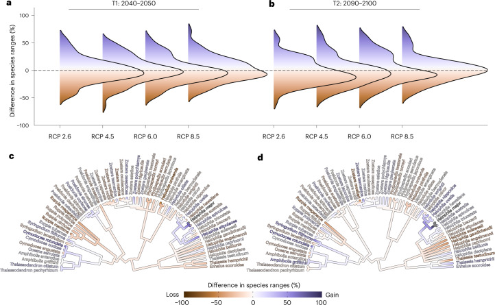
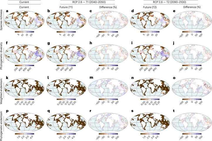
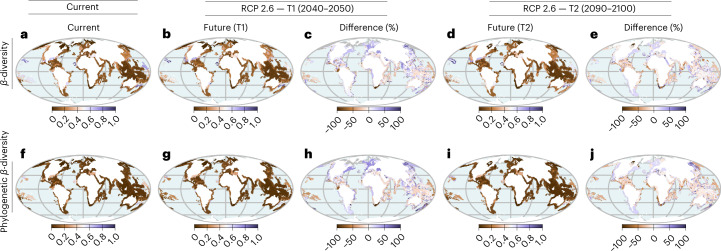
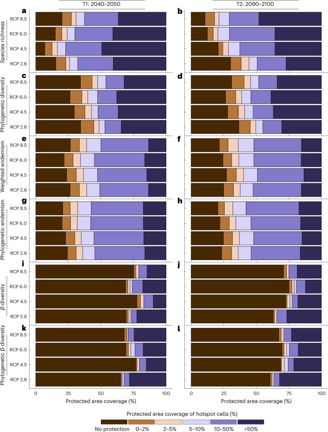
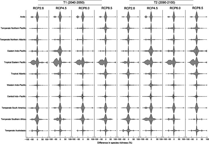
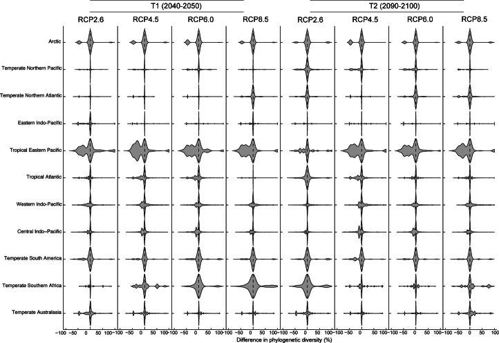
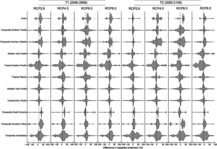
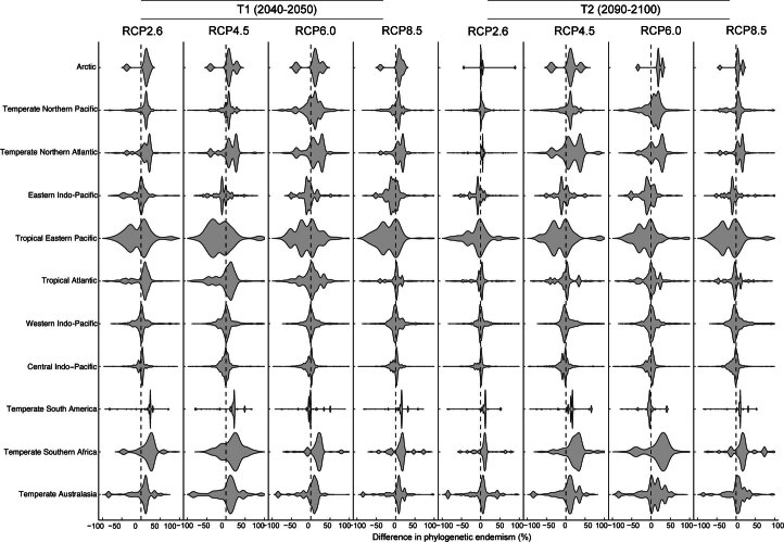
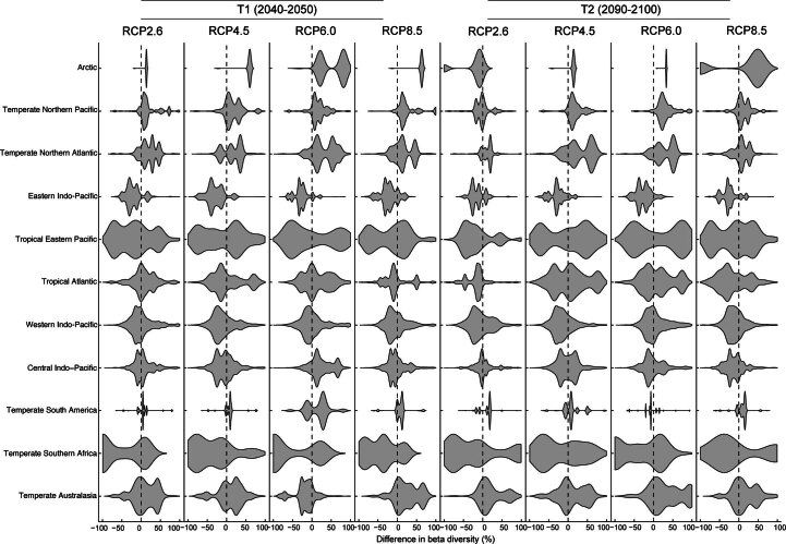
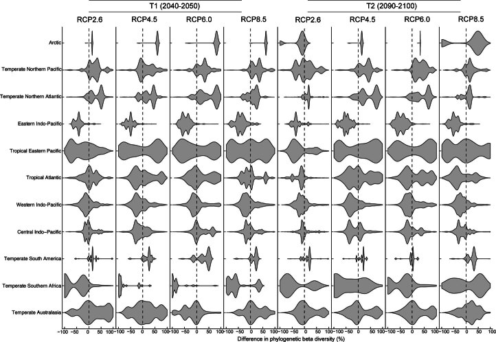
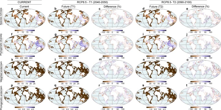
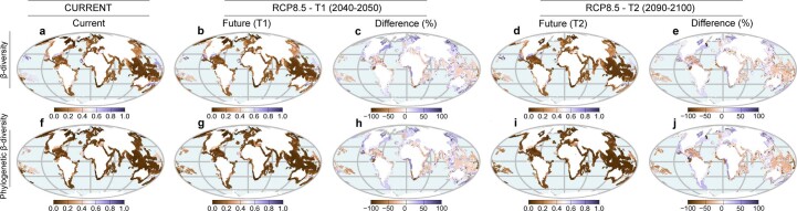
Although climate change projections indicate significant threats to terrestrial biodiversity, the effects are much more profound and striking in the marine environment. Here we explore how different facets of locally distinctive α- and β-diversity (changes in spatial composition) of seagrasses will respond to future climate change scenarios across the globe and compare their coverage with the existing network of marine protected areas. By using species distribution modelling and a dated phylogeny, we predict widespread reductions in species' range sizes that will result in increases in seagrass weighted and phylogenetic endemism. These projected increases of endemism will result in divergent shifts in the spatial composition of β-diversity leading to differentiation in some areas and the homogenization of seagrass communities in other regions. Regardless of the climate scenario, the potential hotspots of these projected shifts in seagrass α- and β-diversity are predicted to occur outside the current network of marine protected areas, providing new priority areas for future conservation planning that incorporate seagrasses. Our findings report responses of species to future climate for a group that is currently under represented in climate change assessments yet crucial in maintaining marine food chains and providing habitat for a wide range of marine biodiversity.

Fig. 1. Taxonomic distribution of seagrass species geographic change at two different time horizons.

For each species, geographic change was estimated using species distribution models fitted using maximum entropy by calculating the percentage of grid cells either lost or gained through time relative to present day. a–d, Estimates of species geographic change were visualized using ridgeline density plots (n = 66 species) for T1 (2040–2050) (a) and T2 (2090–2100) (b) under four different RCPs (2.6, 4.5, 6.0 and 8.5); and phylogenetically (n = 66 species) for T1 (2040–2050) (c) and T2 (2090–2100) (d) for RCP 2.6 (see Supplementary Table 1 for geographic change at other RCPs). Negative values indicate reduction in range size and positive values correspond to range expansions. Dashed horizontal lines in a and b indicate no range change.

Fig. 2. Temporal and geographic patterns of change in α-diversity of seagrasses under climate change.

Estimates are based on species distribution models of seagrasses (n = 66 species) fitted using maximum entropy and aggregated to 100 × 100 km² grid cells. Indicated are the spatial and temporal distributions of: a–e, species richness (number of species in a grid cell) for (a) current, (b) future, and (c) difference for mid-century (2050) and (d) future, and (e) difference forend-of-century (2100); f–j, phylogenetic diversity (sum phylogenetic branch lengths connecting species in a grid cell) for (f) current, (g) future, and (h) difference for mid-century (2050) and (i) future, and (j) difference for end-of-century (2100); and k–o, weighted endemism (species richness inversely weighted by species ranges) for (k) current, (l) future, and (m) difference for mid-century (2050) and (n) future, and (o) difference for end-of-century (2100); p–t, phylogenetic endemism (the amount ofevolutionary history that is unique to a particular areas) for (p) current, (q) future, and (r) difference for mid-century (2050) and (s) future, and (t) difference for end-of-century (2100). Differences in α-diversity for each metric are shown for T1 (2040–2050) and T2 (2090–2100) both under RCP 2.6 (best-case scenario). For each difference map (T1 (c,h,m,r) and T2 (e,j,o,t)), negative values indicate reductions in diversity and positive values correspond to increases in total diversity. Analyses of phylogenetic diversity and phylogenetic endemism were based on a randomly selected subset of 100 trees from a random distribution of 1,000 trees. Projected shifts in α-diversity under different climate scenarios are presented in Extended Data Figs. 1–4. The maps are in the Mollweide projection.

Fig. 3. Geographic and temporal changes in β-diversity in seagrasses under climate change.

a–e, Spatial and temporal changes in species β diversity for (a) current, (b) future, and (c) difference for mid-century (2050) and (d) future, and (e) difference for end-of-century (2100). f–j, Spatial and temporal changes in phylogenetic β diversity for (f) current, (g) future, and (h) difference for mid-century (2050) and (i) future, and (j) difference for end-of-century (2100). Changes in β-diversity were based on species distribution models fitted using maximum entropy and estimated using Simpson dissimilarity index for grid cells across time. Differences in β-diversity for each metric are shown for T1 (2040–2050) and T2 (2090–2100) both under RCP 2.6 (best-case scenario). Positive values in c, e, h and j indicate increasing dissimilarity (differentiation) and negative values correspond to decreasing dissimilarity (homogenization). Temporal and spatial changes in β-diversity were calculated across marine ecoregions of the world. The maps are in the Mollweide projection.

Fig. 4. Overlap of MPAs with future hotspots of α- and β-diversity of seagrasses.

a–l, Indicated are overlaps with hotspots of: species richness (a,b), phylogenetic diversity (c,d), weighted endemism (e,f), phylogenetic endemism (g,h), β-diversity (i,j) and phylogenetic β-diversity (k,l). Overlaps are shown for future hotspots in T1 (2040–2050) (a,c,e,g,i,k) and T2 (2090–2100) (b,d,f,h,j,l) across four different RCPs (2.6, 4.5, 6.0 and 8.5). Overall, only a modest fraction of future hotspots will be contained within MPAs. Analyses of phylogenetic diversity and phylogenetic endemism were based on a randomly selected subset of 100 trees from a random distribution of 1,000 trees.

Extended Data Fig. 1. Temporal changes in species richness of seagrasses under scenarios of climate change.

Estimates of species richness are based on species distribution models of seagrasses (n = 66 species) fitted using maximum entropy and aggregated as number of species in 100 km × 100 km grid cells. Indicated are the differences in species richness across 11 marine ecoregions for four different representative concentration pathways (RCP2.6, 4.5, 6.0, and 8.5) and for two time periods T1: 2040–2050 and T2: 2090–2100. Negative values indicate reductions in species richness and positive values correspond to increases in richness in a region.

Extended Data Fig. 2. Temporal changes in phylogenetic diversity of seagrasses under scenarios of climate change.

Estimates of phylogenetic diversity are based on the species distribution models of seagrasses (n = 66 species) fitted using maximum entropy and aggregated as the sum of phylogenetic branch lengths connecting species in each 100 km × 100 km grid cell. Indicated are the differences in phylogenetic diversity richness across 11 marine ecoregions for four different representative concentration pathways (RCP2.6, 4.5, 6.0, and 8.5) and for two time periods T1: 2040–2050 and T2: 2090–2100. Negative values indicate reductions in phylogenetic diversity and positive values correspond to increases in phylogenetic diversity in a region.

Extended Data Fig. 3. Temporal changes in weighted endemism of seagrasses under scenarios of climate change.

Estimates of weighted endemism are based on the species distribution models of seagrasses (n = 66 species) fitted using maximum entropy and aggregated as species richness inversely weighted by species ranges in each 100 km × 100 km grid cell. Indicated are the differences in weighted endemism across 11 marine ecoregions for four different representative concentration pathways (RCP2.6, 4.5, 6.0, and 8.5) and for two time periods T1: 2040–2050 and T2: 2090–2100. Negative values indicate reductions in weighted endemism and positive values correspond to increases in weighted endemism in a region.

Extended Data Fig. 4. Temporal changes in phylogenetic endemism of seagrasses under scenarios of climate change.

Estimates of phylogenetic endemism are based on the species distribution models of seagrasses (n = 66 species) fitted using maximum entropy and aggregated as phylogenetic diversity restricted to any 100 km × 100 km grid cell. Indicated are the differences in phylogenetic endemism across 11 marine ecoregions for four different representative concentration pathways (RCP2.6, 4.5, 6.0, and 8.5) and for two time periods T1: 2040–2050 and T2: 2090–2100. Negative values indicate reductions in phylogenetic endemism and positive values correspond to increases in phylogenetic endemism in a region.

Extended Data Fig. 5. Temporal changes in species beta diversity of seagrasses under scenarios of climate change.

Estimates of beta diversity are based on the species distribution models of seagrasses (n = 66 species) fitted using maximum entropy and aggregated as the variation in species composition between sites that is, between 100 km × 100 km grid cells. Indicated are the differences in beta diversity across 11 marine ecoregions for four different representative concentration pathways (RCP2.6, 4.5, 6.0, and 8.5) and for two time periods T1: 2040–2050 and T2: 2090–2100. Negative values indicate reductions in beta diversity (that is, species composition will become more identical) and positive values correspond to increases in beta diversity (that is, species composition will become more dissimilar) in the future.

Extended Data Fig. 6. Temporal changes in phylogenetic beta diversity of seagrasses under scenarios of climate change.

Estimates of phylogenetic beta diversity are based on the species distribution models of seagrasses (n = 66 species) fitted using maximum entropy and aggregated as the variation in phylogenetic composition between sites that is, between 100 km × 100 km grid cells. Indicated are the differences in phylogenetic beta diversity across 11 marine ecoregions for four different representative concentration pathways (RCP2.6, 4.5, 6.0, and 8.5) and for two time periods T1: 2040–2050 and T2: 2090–2100. Negative values indicate reductions in phylogenetic beta diversity (that is, phylogenetic composition will become more identical) and positive values correspond to increases in beta diversity (species composition will become more dissimilar) in the future.

Extended Data Fig. 7. Temporal and geographic patterns of change in alpha diversity of seagrasses under a worst-case scenario of climate change.

Estimates are based on species distribution models of seagrasses (n = 66 species) fitted using maximum entropy and aggregated to 100 km × 100 km grid cells. Indicated are the spatial and temporal changes between current and future distributions of α-diversity based on: a–e, species richness (number of species in a grid cell), f–j, phylogenetic diversity (sum of phylogenetic branch lengths connecting species in a grid cell), k–o, weighted endemism (species richness inversely weighted by species ranges), and, p–t, phylogenetic endemism (the amount of evolutionary history that is unique to a particular area). Differences in α-diversity for each metric are shown for T1: 2040–2050 and T2: 2090–2100 both under RCP8.5 (worst-case scenario). For each difference map (T1: c, h, m, r, and T2: e, j, o, t), negative values indicate reductions in diversity and positive values correspond to increases in total diversity. Analyses of phylogenetic diversity and phylogenetic endemism were based on a randomly selected subset of 100 trees from a random distribution of 1000 trees.

Extended Data Fig. 8. Geographic and temporal changes in beta diversity in seagrasses under a worst-case scenario of climate change.

a–e Spatial and temporal changes in species (β) diversity. f–j Spatial and temporal changes in phylogenetic (β) diversity. Changes in beta diversity were based on species distribution models fitted using maximum entropy and estimated using Simpson dissimilarity index for grid cells across time. Differences in β-diversity for each metric are shown for T1: 2040–2050 and T2: 2090–2100 both under RCP8.5 (worst-case scenario). Positive values in c, e, h, and j indicate increasing dissimilarity (differentiation) and negative values correspond to decreasing dissimilarity (that is, homogenization). Temporal and spatial changes in beta diversity were calculated across marine ecoregions of the world. The maps are in the Mollweide projection.

References

1. Burrows MT, et al. The pace of shifting climate in marine and terrestrial ecosystems. Science. 2011;334:652–655. - PubMed
1. Blowes SA, et al. The geography of biodiversity change in marine and terrestrial assemblages. Science. 2019;366:339–345. - PubMed
1. Jabbour J, Hunsberger C. Visualizing relationships between drivers of environmental change and pressures on land-based ecosystems. Nat. Resour. 2014;5:146–160.
1. Elahi R, et al. Recent trends in local-scale marine biodiversity reflect community structure and human impacts. Curr. Biol. 2015;25:1938–1943. - PubMed
1. Zeebe R, Ridgwell A, Zachos J. Anthropogenic carbon release rate unprecedented during the past 66 million years. Nat. Geosci. 2016;9:325–329.
Publication types