Effects of Hallucination Proneness and Sensory Resolution on Prior Biases in Human Perceptual Inference of Time Intervals

Abstract

Bayesian models of perception posit that percepts result from the optimal integration of new sensory information and prior expectations. In turn, prominent models of perceptual disturbances in psychosis frame hallucination-like phenomena as percepts excessively biased toward perceptual prior expectations. Despite mounting support for this notion, whether this hallucination-related prior bias results secondarily from imprecise sensory representations at early processing stages or directly from alterations in perceptual priors-both suggested candidates potentially consistent with Bayesian models-remains to be tested. Using modified interval timing paradigms designed to arbitrate between these alternative hypotheses, we show in human participants (16 females and 24 males) from a nonclinical population that hallucination proneness correlates with a circumscribed form of prior bias that reflects selective differences in weighting of contextual prior variance, a prior bias that is unrelated to the effect of sensory noise and to a separate index of sensory resolution. Our results thus suggest distinct mechanisms underlying prior biases in perceptual inference and favor the notion that hallucination proneness could reflect direct alterations in the representation or use of perceptual priors independent of sensory noise.SIGNIFICANCE STATEMENT Current theories of psychosis posit that hallucination proneness results from excessive influence of prior expectations on perception. It is not clear whether this prior bias represents a primary top-down process related to the representation or use of prior beliefs or instead a secondary bottom-up process stemming from imprecise sensory representations at early processing stages. To address this question, we examined interval timing behaviors captured by Bayesian perceptual-inference models. Our data support the notion that excessive influence of prior expectations associated with hallucination propensity is not directly secondary to sensory imprecision and is instead more consistent with a primary top-down process. These results help refine computational theories of psychosis and may contribute to the development of improved intervention targets.

Keywords: hallucinations; interval timing; perceptual inference; prior beliefs; psychosis; sensory resolution.

Figure 1.

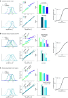
Schematic of temporal categorization and interval timing tasks. Task 1, Interval timing. a, Schematic of the trial structure for the interval timing task. Subjects reproduced the sample interval (sample time) demarcated by the time between two brief flashes, Ready and Set, via a key press so that the production time was the time between the Set flash and key press. b, c, Four uniform prior distributions of sample intervals were used to manipulate either sensory noise by changing (b) the mean interval length (NS, NM, and NL) or the prior variance by changing (c) the interval width (NM, WM). Right, Distributions of sample intervals. In each session, sample intervals were drawn randomly from one of these distributions. Middle, Hypothesized results show increased central tendency (decreased slopes relating sample times to production times) as a function of mean interval length (length effect), indicating sensitivity to sensory noise (which increases with interval length, as expected according to the scalar variability principle) and decreased central tendency with increased interval width (width effect), indicating sensitivity to prior variance. Task 2, Temporal categorization. d, Schematic of the trial structure for the temporal categorization task. Subjects performed a two-interval forced-choice task in which, after a random delay (1–2 s) following the appearance of a fixation dot, the first fixed interval was defined as the time in between two brief flashes. The second interval was defined as the time between the second and the third flashes, determined by a QUEST adaptive algorithm. Subjects then decided whether the first or the second interval was longer by pressing the corresponding key. e, Example of a fitted psychometric curve derived from the temporal categorization task illustrating the two measures of interest, the PSE and the WF, an index of sensory resolution (higher WF values indicate a more shallow slope and lower resolution).

Figure 2.

Simulations from the BLS model illustrating length and width effects on interval timing and their changes under decreased sensory resolution (higher WF) and altered representation of prior variance. a–c, Baseline (unaltered) model predictions with a WF of 0.1, indicating relatively high sensory resolution representative of the average subject in our sample. Slopes, inversely proportional to central tendency, decrease with increasing mean interval length (length effect) and increase with increasing interval width (width effect), respectively, indicating increased reliance on prior expectations with increased sensory noise and with decreased prior variance. To facilitate comparisons with the baseline model predictions in b and c, we show the baseline predictions of the unaltered model in lighter colors. Model predictions with decreased sensory resolution (WF = 0.2) are shown in darker colors (b). The central tendency values in all conditions increase (slopes decrease) relative to the baseline model in a. Model predictions with constrained representation of prior variance (c), simulated as a reduction of the variance in the wide-medium condition; WF of 0.1 (sensory resolution as in a) is shown in darker colors. The central tendency in the wide-medium condition is selectively increased (slopes decreased). The BLS model returns a posterior probability by combining the statistics of the environment as a Bayesian prior with a given likelihood (a–c). For illustration purposes only, the uniform distributions are transformed into Gaussian distributions (with the SD equal to the width of the uniform distribution divided by the root mean square of 12); the nonlinear output of the BLS is approximated by a linear function that intersects with the identity line at the indifference point and whose slope inversely correlates with the central tendency. Psychometric functions are cumulative Gaussians with slope representing the corresponding WF. Motor noise is set to 0.1 in all cases.

Figure 3.

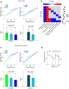
Group and individual data demonstrate length and width effects on interval timing. Top, Group-level results. a, Slopes showing central tendency differences by condition (length and width effects). For visualization of results, slopes are obtained by least-squares regression of group means of mean individual responses for each bin. Error bars indicate SEM for the group for each bin. Bar plots indicate mean slopes from regression of mean individual responses for each bin. Error bars indicate SEM of the group; *p ≤ 0.05. b, Matrix showing t statistics of fixed effects from LME for models with increasing complexity (from model 1 to model 8, with increasing number of covariates adjusting for nonstationarity effects) in the y-axis. Big or small white asterisks within the cells indicate statistically significant at p ≤ 0.001 or at p ≤ 0.05, respectively, for a given variable (x-axis). Right, Marginal plot on the right indicates AIC and BIC for each model, with the arrow indicating the winning model based on LRT, which coincides with the lowest (best) AIC and BIC. c) and d) Representative individual (condition order WM-NM-NS-NL, WF = 0.08, CAPS = 0). c, Slopes showing central tendency differences by condition (length and width effects). Slopes are obtained by least-squares regression of mean individual responses per bin. Error bars indicate SE across responses. Bar plots show slopes and error bars indicate SEM for the regression coefficients. d, Changes in central tendency over trials (instantaneous slopes) estimated from a sliding window of 43 trials in a linear regression model illustrating nonstationarity effects; instability of slopes is shown at the beginning of the task (start effect) and at transition points between conditions (indicated by vertical lines; transition effects).

Figure 4.

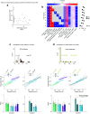
Interindividual effects of sensory resolution measured as WF, and hallucination proneness (CAPS) on central tendency, length, and width effects. a, Scatter plot showing a nonsignificant relationship between CAPS scores and WF across subjects. b, t Statistics showing fixed-effect results from LME models (conventions as in Fig. 3a). The winning model (model 8) is selected based on AIC, BIC, and LRT (arrow). Extended Data Fig. 4-1 depicts the t statistics obtained from these LME models applied to data from the last two blocks for each condition. c, Mean slopes showing no significant central tendency differences by WF level (low vs high in light vs dark colors; ≤30th versus ≥70th percentile, respectively) and condition (length and width effects). d, Mean adjusted slopes showing central tendency differences by CAPS level (low vs high in light vs dark colors; ≤61st or ≥80th percentile, respectively; see above, Materials and Methods) and condition (length and width effects). The significant effect of CAPS on width effects in b appears to be driven by a selective increase in central tendency (decreased slopes) in the wide-medium (WM) condition. Mean slopes are obtained by least-squares regression of group means of mean individual responses for each bin. Error bars indicate SEM for the group for each bin. For robustness, bar plots for c and d show mean of slopes from least-square regression of mean individual responses for each bin, adjusted for the variable of no interest to isolate effects of interest for each variable (i.e., for WF, slopes are adjusted by CAPS, and for CAPS, they are adjusted by WF). Error bars indicate SEM for the group.

References

1. Acerbi L, Wolpert DM, Vijayakumar S (2012) Internal representations of temporal statistics and feedback calibrate motor-sensory interval timing. PLoS Comput Biol 8:e1002771. 10.1371/journal.pcbi.1002771 - DOI - PMC - PubMed
1. Adams RA, Stephan KE, Brown HR, Frith CD, Friston KJ (2013) The computational anatomy of psychosis. Front Psychiatry 4:47. 10.3389/fpsyt.2013.00047 - DOI - PMC - PubMed
1. Akaike H (1974) A new look at the statistical model identification. IEEE Trans Automat Contr 19:716–723. 10.1109/TAC.1974.1100705 - DOI
1. Alderson-Day B, Lima CF, Evans S, Krishnan S, Shanmugalingam P, Fernyhough C, Scott SK (2017) Distinct processing of ambiguous speech in people with non-clinical auditory verbal hallucinations. Brain 140:2475–2489. 10.1093/brain/awx206 - DOI - PubMed
1. Ashourian P, Loewenstein Y (2011) Bayesian inference underlies the contraction bias in delayed comparison tasks. PLoS One 6:e19551. 10.1371/journal.pone.0019551 - DOI - PMC - PubMed
Publication types