A Database of Snow on Sea Ice in the Central Arctic Collected during the MOSAiC expedition

Abstract

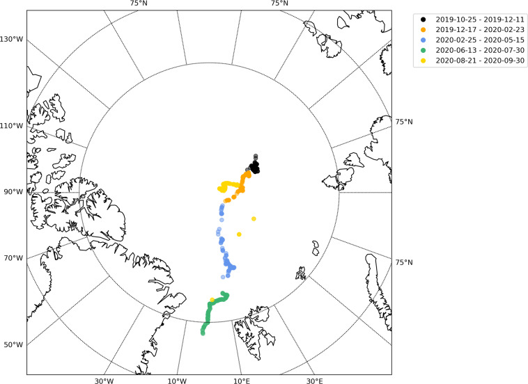
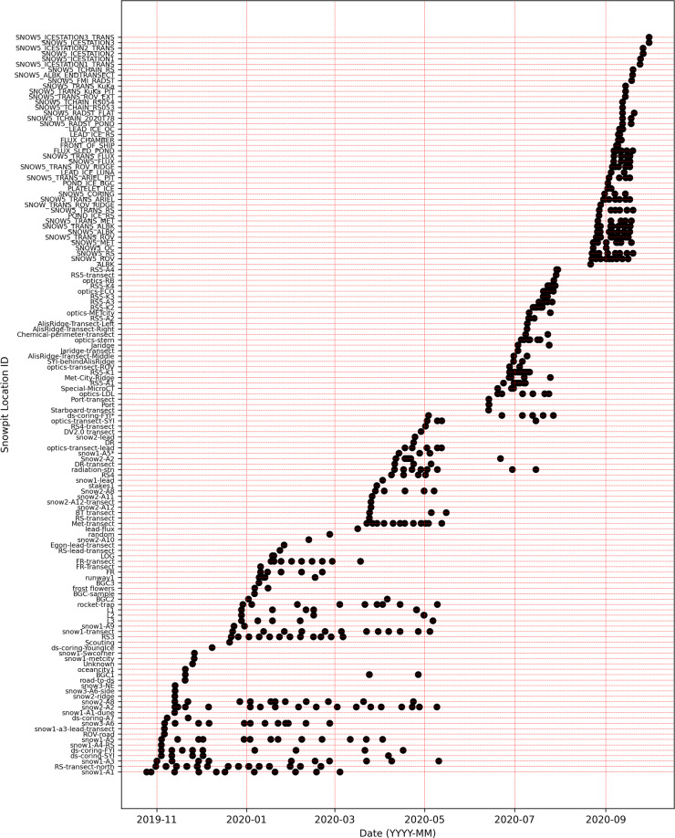
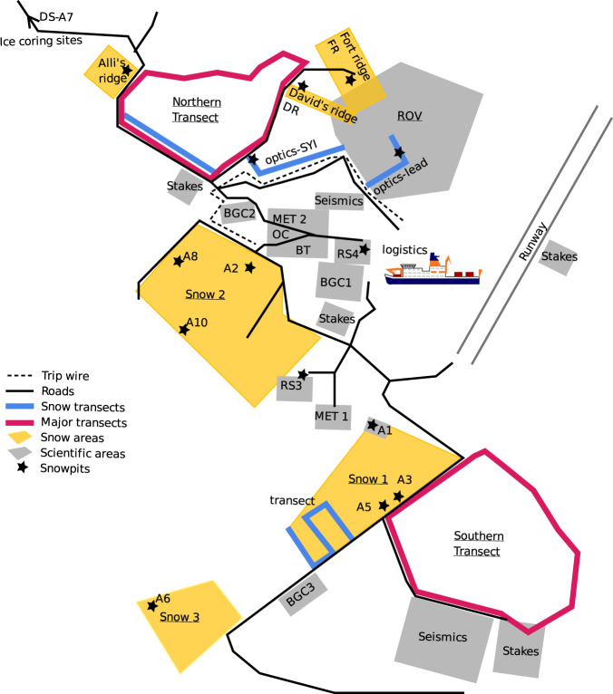
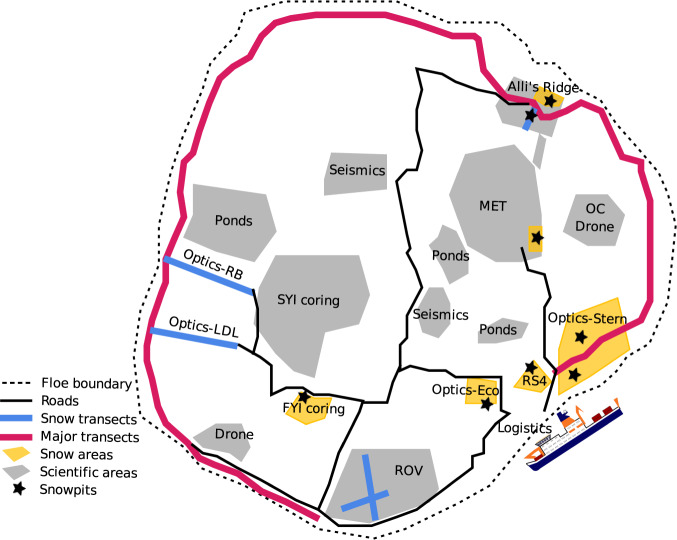
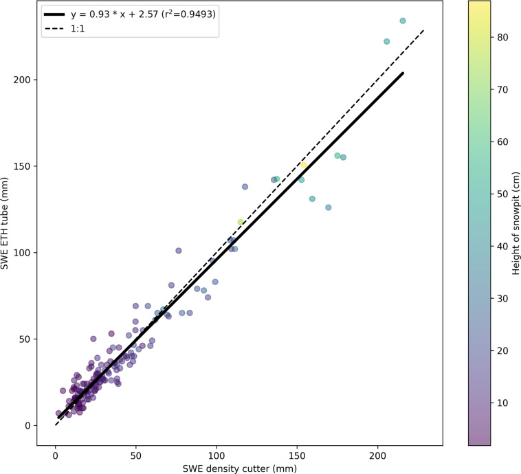
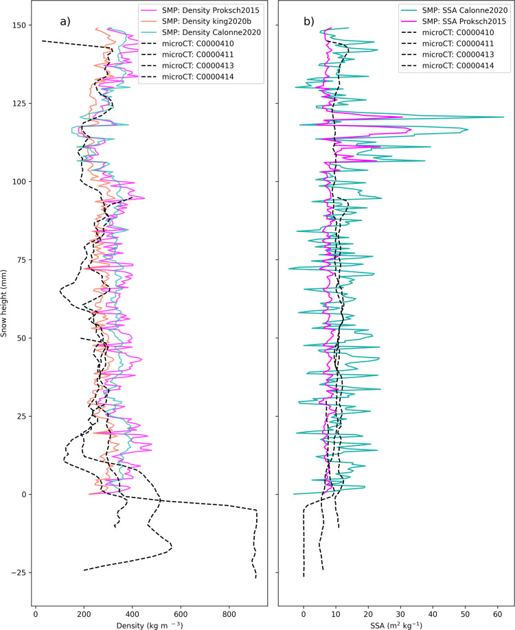
Snow plays an essential role in the Arctic as the interface between the sea ice and the atmosphere. Optical properties, thermal conductivity and mass distribution are critical to understanding the complex Arctic sea ice system's energy balance and mass distribution. By conducting measurements from October 2019 to September 2020 on the Multidisciplinary drifting Observatory for the Study of Arctic Climate (MOSAiC) expedition, we have produced a dataset capturing the year-long evolution of the physical properties of the snow and surface scattering layer, a highly porous surface layer on Arctic sea ice that evolves due to preferential melt at the ice grain boundaries. The dataset includes measurements of snow during MOSAiC. Measurements included profiles of depth, density, temperature, snow water equivalent, penetration resistance, stable water isotope, salinity and microcomputer tomography samples. Most snowpit sites were visited and measured weekly to capture the temporal evolution of the physical properties of snow. The compiled dataset includes 576 snowpits and describes snow conditions during the MOSAiC expedition.

Fig. 1

Snowpit locations of each unique device operation ID. A map showing the latitude and longitude of each snowpit visit from 2019-10-25 to 2020-09-30. Each device operation ID is indicated by one mark on the figure and the colours represent the time period for each device operation ID beginning with PS122/1, PS122/2, PS122/3, PS122/4 and PS122/5 respectively. Refer to the usage notes to relate the device operation ID to the dates of interest and the contact person. The marks have transparency so the darker marks represent multiple measurements in one coordinate region.

Fig. 2

Time series of snowpit measurements at each snowpit site. A black mark indicates one visit to the snowpit site. The name of the snowpit site is indicated on the y-axis. The relocation of the central observatory and ice dynamics can be seen through the discontinuation of certain time series. This figure is to visualise the overall snowpit time series. However, due to the limited font size, please refer to the metadata publication for detailed information on specific dates of the snowpit site visits.

Fig. 3

Schematic diagram of the snowpit locations across central observatory 1. Schematic diagram of central observatory 1 (CO1) adapted from the maps used during the expedition from 2019-10-25 - 2020-05-15. For detailed information on location acronyms, please refer to the snow and ice overview manuscript.

Fig. 4

Schematic diagram of the snowpit locations across central observatory 2. Schematic diagram of central observatory 2 (CO2) adapted from the maps used during the expedition from 2020-06-13 - 2020-07-30. For detailed information on location acronyms, please refer to the snow and ice overview manuscript.

Fig. 5

Schematic diagram of the snowpit locations across central observatory 3. Schematic diagram of central observatory 3 (CO3) adapted from the maps used during the expedition from 2020-08-21 - 2020-09-30 after the relocation of Polarstern. For detailed information on location acronyms, please refer to the snow and ice overview manuscript.

Fig. 6

A combination of the different instruments taken to the snowpit site. (a) An example overview picture, photo credits with publishing permission: A. Macfarlane. (b) The micro-CT mounted in the cold laboratory on Polarstern. A snow sample is being held in the white sample holder of 88 mm diameter; other sizes of samples can be seen in the table on the right side of the image, photo credits with publishing permission M. Jaggi. (c) The SWE tube and the ruler in the snowpit in the spring season, photo credits with publishing permission: A. Macfarlane. (d) The SWE tube in action in the field, photo credits with publishing permission: M. Jaggi. (e) The SMP measuring penetration resistance in front of an ice ridge. photo credits with publishing permission: D. Ruché. (f) The NIRbox taking an image of the snowpit wall, photo credits with publishing permission: M. Jaggi. (g) A density cutter (left of the ruler) and thermometer (right of the ruler) inserted in the snowpit wall, photo credits with publishing permission: A. Macfarlane. (h) An SfM example image showing the SfM targets placed on the naturally illuminated snow surface, photo credits with publishing permission: A. Macfarlane. (i) An SfM example image showing the SfM targets placed on the snow-ice interface; this image is illuminated using a head torch in the field, photo credits with publishing permission: M. Schneebeli.

Fig. 7

A case study of the measurements taken during event ID PS122/3_37-41. The overview image in the background of (A) gives an example of the conditions upon arrival at the snowpit. Annotations to this image show the different measurement locations and their relation to each other. The pink highlighted box shows the surface roughness measurement (SfM) location and the snowpit excavation area to allow access to the snowpit wall. Once excavated, the yellow box shows where the core measurements are taken, listed as bullet points. (B) shows the excavated pit revealing the underlying sea ice surface, also measured for roughness using SfM. The red points indicate the SMP measurements. The five central SMP measurements are located in the snowpit, and to capture spatial heterogeneity, sometimes additional measurements were conducted to the left and right of the snowpit. (C) shows the SMP force signals over depth with the categorised grain types. This gives an indication of the spatial heterogeneity within the snowpit. The image in (D) is from the NIRbox during device operation ID PS122/3_36-138. The annotations of this figure show the reference targets (95 and 50%) and the NIRbox frame above the excavated snowpit wall.

Fig. 8

Time series of parameters for the entire season. This figure gives an overview of the published datasets on Pangaea covering the entire season and collected on all three central observatories (CO1, CO2 and CO3). One marker in these graphs indicates one measurement. The marks have transparency, so the darker marks represent multiple measurements at one timestamp. (a,c) show a temperature time series taken at different heights in the snowpack. (b,d) show measurements of snow density using the density cutter, where one point represents one cutter measurement. (e) shows the SWE tube time series, (f) shows the salinity time series, and finally, (g) shows the stable water isotope δ¹⁸O time series.

Fig. 9

SWE parameter cross-checked against ETH tube measurement and density cutter measurements. At each snowpit, it was common to take measurements of SWE using the aluminium SWE ETH-tube and density using the density cutter. By using the equation linking SWE to the density and volume of snow, we are able to compare the two instruments. This figure presents a SWE comparison of the SWE ETH-tube to the SWE calculated using the density cutter covering measurements of the entire season and collected on all three central observatories (CO1, CO2 and CO3). The average of all density cutter measurements in one profile was multiplied by the corresponding height in the SWE-ETH tube to obtain the SWE for the density cutter. The SWE-ETH tube values were taken directly from the dataset. If there were multiple measurements for one profile, the average SWE was taken.

Fig. 10

A co-location of SMP and micro-CT measurements for device operation ID PS122/3_38-94. (a) Shows density derived from the micro-CT and SMP parameterisations; Proksch2015, King2020b and Calonne2020. (b) shows SSA derived from the micro-CT and SMP parameterisations; Calonne2020 and Proksch2015. This figure highlights the importance of taking care when choosing the density and SSA parameterisations in all future analyses of this dataset.

References

1. Eicken H, Fischer H, Lemke P. Effects of the snow cover on Antarctic sea ice and potential modulation of its response to climate change. Annals of Glaciology. 1995;21:369–376. doi: 10.3189/S0260305500016086. - DOI
1. Fichefet T, Maqueda M. Modelling the influence of snow accumulation and snow-ice formation on the seasonal cycle of the Antarctic sea-ice cover. Climate Dynamics. 1999;15:251–268. doi: 10.1007/s003820050280. - DOI
1. Massom RA, et al. Snow on Antarctic sea ice. Reviews of Geophysics. 2001;39:413–445. doi: 10.1029/2000RG000085. - DOI
1. Lecomte O, Fichefet T, Flocco D, Schroeder D, Vancoppenolle M. Interactions between wind-blown snow redistribution and melt ponds in a coupled ocean-sea ice model. Ocean Modelling. 2015;87:67–80. doi: 10.1016/j.ocemod.2014.12.003. - DOI
1. Lecomte O, et al. On the formulation of snow thermal conductivity in large-scale sea ice models. Journal of Advances in Modeling Earth Systems. 2013;5:542–557. doi: 10.1002/jame.20039. - DOI