Electrochemical Impedance Spectroscopy-A Tutorial

Abstract

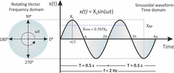
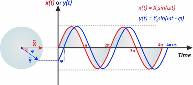
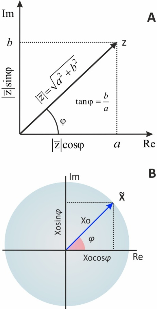
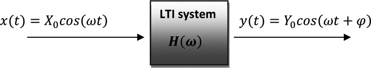
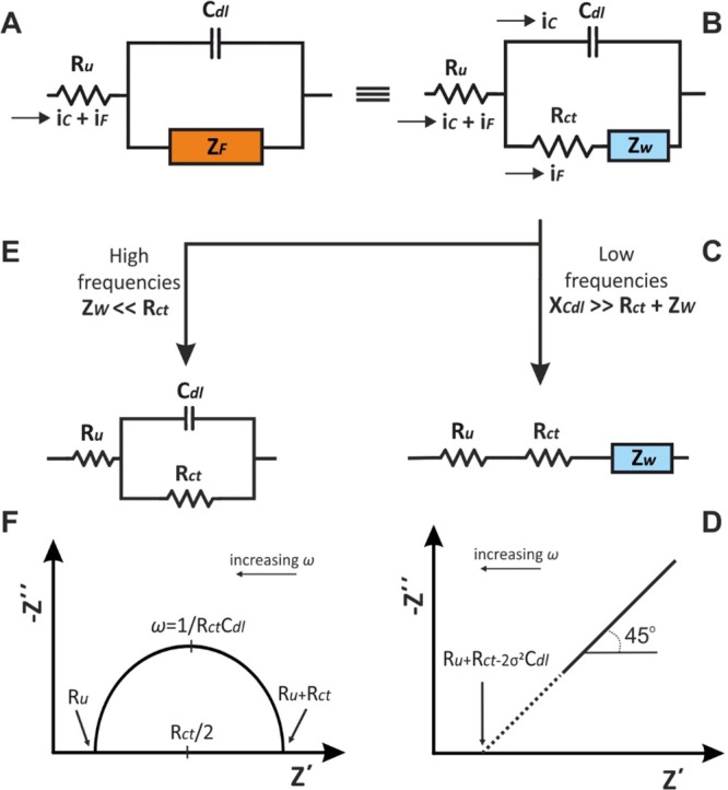
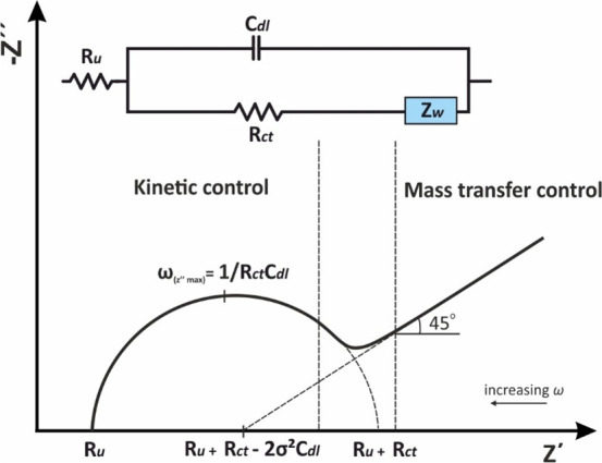
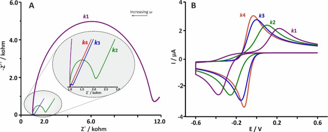
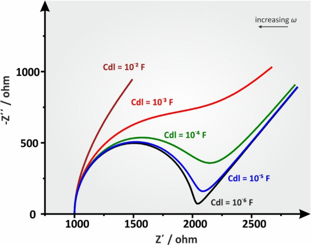
This tutorial provides the theoretical background, the principles, and applications of Electrochemical Impedance Spectroscopy (EIS) in various research and technological sectors. The text has been organized in 17 sections starting with basic knowledge on sinusoidal signals, complex numbers, phasor notation, and transfer functions, continuing with the definition of impedance in electrical circuits, the principles of EIS, the validation of the experimental data, their simulation to equivalent electrical circuits, and ending with practical considerations and selected examples on the utility of EIS to corrosion, energy related applications, and biosensing. A user interactive excel file showing the Nyquist and Bode plots of some model circuits is provided in the Supporting Information. This tutorial aspires to provide the essential background to graduate students working on EIS, as well as to endow the knowledge of senior researchers on various fields where EIS is involved. We also believe that the content of this tutorial will be a useful educational tool for EIS instructors.

Figure 1

Representation of a vector rotating with a constant angular frequency ω and the corresponding sinusoidal signal, x(t) = X_o sin(ωt).

Figure 2

Phasor diagrams for the sinusoidal signals x(t) and y(t). The immobile vectors after a specific time correspond to the phasors X̃ and Ỹ and the phase difference between them.

Figure 3

Representation of a (A) complex number z and a (B) phasor X̃ on the complex plane

Figure 4

Schematic representation of a linear time-invariant (LTI) system with an input sinusoidal signal x(t) at a frequency ω and the output sinusoidal signal y(t) at the same frequency. The input/output signals are related with the transfer function H(ω).

Figure 5

(Left) phasor diagrams and (right) the respective sinusoidal waveforms v(t) and i(t) when a low amplitude alternating voltage is applied to (A) a resistor, (B) a capacitor, and (C) an inductor.

Figure 6

(A) Schematic representation of an electrochemical system’s response to a low-amplitude (V_o) sinusoidal signal superimposed to a constant voltage V_dc and (B) the respective Lissajous plots if we consider that the phase shift between the perturbating and response alternating signals is 0°, 45°, or 90°. (C) A Lissajous plot showing a nonlinear response. Courtesy of Metrohm Autolab B.V. (D) Lissajous plots of a system interrogated with an ac voltage with amplitude ±10 mV, at 20 Hz, where the amplitude of the current response decreases with time. Reprinted in part with permission from ref (31). Copyright 2021 Wiley.

Figure 7

Examples of different electrical circuits that generate identical impedance spectra.

Figure 8

Nyquist, Bode magnitude and phase angle plots of some model circuits. R1 = 1 kOhm.

Figure 9

Nyquist, Bode magnitude, and phase angle plots of some model circuits. R0 = R1 = R2 = 1 kOhm.

Figure 10

Simplified experimental setup for potentiostatic EIS and working principle of a frequency response analyzer. “X”, stands for multipliers and “∫” for integrators.

Figure 11

Accuracy contour plot indicating that within the blue area and under specific experimental conditions, impedance and phase angle readings are recorded with a maximum error 0.3% and 1°, respectively. Outside this area and within the gray area, the errors increase up to 2% and 3°, respectively. Errors’ values are given as an example.

Figure 12

Different types of electrochemical cells of 2-, 3-, and 4-electrodes and different connection modes with the working (WE), working sense (WS), counter (CE), and reference (RE) electrodes.

Figure 13

(A, B) The Randles equivalent circuit and its behavior at (C, D) low and (E, F) high frequencies. Adapted with permission from ref (4). Copyright 2022 Wiley.

Figure 14

Randles equivalent electrical circuit over a wide frequency range.

Figure 15

(A) Nyquist plots for an electrochemical process involving a redox reaction at different R_ct corresponding to different heterogeneous transfer kinetics rates (k⁰) and (B) the respective cyclic voltammograms at the same k⁰ values. R_u = 1 kOhm, C_dl = 10^–6 F, and Z_w = 10^–2 Ohm^–1/2 s^1/2.

Figure 16

Simulated Nyquist plots of a R_u(C_dl[R_ctZ_w]) circuit at different C_dl values. R_u = 1 kOhm, R_ct = 1 kOhm, and Z_w = 10^–2 Ohm^–1/2 s^1/2.

Figure 17

Nyquist plots for CPE at (A) R_uC_dl and (B) R_u(C_dlR_ct) circuits.

Figure 18

(A) The semi-infinite regime of an electrochemical cell, (B) the transmission line (TL) depiction of the semi-infinite regime, (C) finite boundary diffusion at t < t_d spans, (D) transmissive, and (E) reflective boundary at t > t_d.

Figure 19

Stylized sketches of total impedance Nyquist plots at different mass transfer regimes.

Figure 20

Simulated Nyquist plot of an RDE experiment with increasing angular velocity (ω) values, leading to increasing B values. R_u = 1000 Ohm, C_dl = 10^–6 F, R_ct = 1000 ohm, Y⁰ = 10^–4 s^1/2 ohm^–1, B = 5.222 s^–1 (ω = 10 rpm), B = 2.335 s^–1 (ω = 50 rpm), B = 1.651 s^–1 (ω = 100 rpm), B = 1.348 s^–1 (ω = 150 rpm), B = 0.953 s^–1 (ω = 300 rpm), B = 0.674 s^–1 (ω = 600 rpm), and B = 0.477 s^–1 (ω = 1200 rpm). D was deemed to be 7.6 × 10^–6, as per the well-known redox couple ferro/ferricyanide, and ν was 0.01 cm² s^–1, which is the approximate value of water’s kinematic viscosity at 25 °C.

Figure 21

Simulated Nyquist plots of an ideal electrode surface with a reflective boundary at various (from 0.5 to 5 s^–1) B values. R_u = 1000 ohm, C_dl = 10^–6 F, R_ct = 1000 ohm, Y⁰ = 10^–3 s^1/2 ohm^–1.

Figure 22

Simulated Nyquist plot of an ideal electrode surface at various (from 0.01 to 10 s^–1) reaction rate values (k_a). R_u = 1000 Ohm, C_dl = 10^–6 F, R_ct = 1000 Ohm, Y⁰ = 10^–4 s^1/2 ohm^–1.

Figure 23

Adapted illustration of De Levie’s model for a flooded porous electrode (A) in the absence and (B) in the presence of a redox molecule.

Figure 24

Suggested connections to alleviate inductive behavior due to (A) the high impedance of the reference electrode and (B) mutual inductance between WE-CE and RE-WS leads.

Figure 25

Nyquist impedance spectra for the iron electrode in 0.5 M H₂SO₄ solution at various potentials. (a) Corrosion potential, −530 mV (vs SCE); (b) −450 mV; (c) −400 mV; (d) −350 mV. Reprinted with permission from ref (77). Copyright 2002 Elsevier.

Figure 26

(A) 2-terminal and 4-terminal connections of a 2-electrode cell with the potentiostat and (B) the respective Nyquist plots adapted from ref. Courtesy of Metrohm Autolab B.V.

Figure 27

(A) Description of individual cell components with equivalent circuit elements. Reprinted with permission from ref (91). Copyright 2016 Wiley. (B) Equivalent circuit model of a lithium-ion half-cell system. Reprinted with permission from ref (93). Copyright 2004 Elsevier.

Figure 28

(A) Nyquist plot of Li|ILE|SE|Li (green line) cell with its respective fit and characteristic peak frequencies. (B) Schematic of the Li|ILE|SE|Li cell and the equivalent circuit used for fitting the impedance data. Li, Lithium electrode, SE, solid electrolyte, ILE, ionic liquid electrolyte, ECR, electrochemical reaction. Adapted with permission from ref (85). Copyright 2021 Wiley.

Figure 29

(A) Schematic of the working principle of a SOFC based on an oxygen ion conducting solid electrolyte. (B) Sketch of the situation where the anode microstructure is modeled as stainless-steel columns coated with a Ce_0.8Gd_0.2O_1.9 (CGO) based infiltration and the electrochemical profile can be described by a transmission line. Reprinted with permission from ref (104). Copyright 2012 Elsevier. (C) CNLS-fit of impedance data to an equivalent electrical circuit that was developed by a preidentification of the impedance response by calculating and analyzing the corresponding distribution of relaxation times (DRT). Reprinted with permission from ref (103). Copyright 2013 Elsevier.

Figure 30

(A) Schematic representation of a DSSC and (B) current–voltage plot of a DSSC. The gray area denotes the voltage perturbation around OCP and the current perturbation around I_sc defining the examined IMVS and IMPS areas under modulated light intensity (C) A simplified experimental setup for the generation of modulated light intensities and cables connection at IMPS and IMVS measurements (D) Imaginary component −Z″(IMVS) of the IMVS transfer function versus the frequency range from 10 kHz to 100 mHz at three light intensities 5 (blue dots), 10 (red dots), and 50 mW/cm² (green dots) with a DSSC, using the N719 dye. Courtesy of Metrohm Autolab B.V.

Figure 31

Schematic representation of a capacitive biosensor showing the buildup of the biosensor and the biorecognition event where the total capacitance is described by various capacitors in series. C_dl, capacitance of the electric double layer; IL, insulating layer; Ab, antibody; Ag, antigen (the target analyte).

Figure 32

(A) Tentative view of the different modification and recognition steps of the BSA-blocked Au/MUAM-MH/GA/Anti-SA immunosensors and (B) Nyquist plots showing the impedimetric response of the immunosensor (a) before and after its incubation with (b) E. coli and (c) S. typhimurium culture samples for 1 h. Initial concentration of bacteria, 10⁶ cfu mL^–1. Measuring conditions, 0.1–10⁵ Hz at +0.200 V bias (10 mV rms). Electrolyte, 5 mM hexacyanoferrate(II)/(III) (1 + 1 mixture) in PBS solution, pH 7. MUAM, 11-Amino-1-undecanethiol hydrochloride; MH, 6-Mercapto-1-hexanol; GA, glutaraldehyde. Reprinted with permission from ref (86). Copyright 2008 ACS Publications.

References

1. Barsoukov E.; MacDonald J. R.. Impedance Spectroscopy: Theory, Experiment, and Applications, 2nd ed.; Wiley-VCH, 2018.
1. Orazem M. E.; Tribollet B. A Tutorial on Electrochemical Impedance Spectroscopy. ChemTexts 2020, 6 (2), 12.10.1007/s40828-020-0110-7. - DOI
1. Orazem M.; Tribollet B.. Electrochemical Impedance Spectroscopy, 2nd ed.; Wiley-VCH, 2008.
1. Bard A. J.; Faulkner L. R.; White H. S.. Electrochemical Methods: Fundamentals and Applications; Wiley-VCH, 2022.
1. Brett C. M. A.; Brett A. M. O.. Electrochemistry Principles, Methods and Applications; Oxford University Press, 1994. 10.1515/bmte.1999.44.s2.11. - DOI