Patterns and determinants of the global herbivorous mycobiome

Abstract

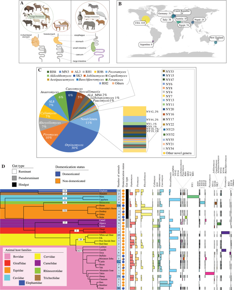
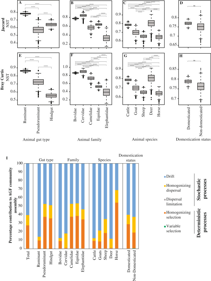
Despite their role in host nutrition, the anaerobic gut fungal (AGF) component of the herbivorous gut microbiome remains poorly characterized. Here, to examine global patterns and determinants of AGF diversity, we generate and analyze an amplicon dataset from 661 fecal samples from 34 mammalian species, 9 families, and 6 continents. We identify 56 novel genera, greatly expanding AGF diversity beyond current estimates (31 genera and candidate genera). Community structure analysis indicates that host phylogenetic affiliation, not domestication status and biogeography, shapes the community rather than. Fungal-host associations are stronger and more specific in hindgut fermenters than in foregut fermenters. Transcriptomics-enabled phylogenomic and molecular clock analyses of 52 strains from 14 genera indicate that most genera with preferences for hindgut hosts evolved earlier (44-58 Mya) than those with preferences for foregut hosts (22-32 Mya). Our results greatly expand the documented scope of AGF diversity and provide an ecologically and evolutionary-grounded model to explain the observed patterns of AGF diversity in extant animal hosts.

Fig. 1. Broad AGF diversity patterns in the herbivorous gut.

A Overview of the anatomy of the GIT tract of various types of herbivores. Colorized parts of the GIT indicate main location of plant fermentation for each gut type. B Map showing the geographical locations and the number of fecal samples analyzed in this study. C Pie chart showing the total percentage abundance of various AGF genera identified in the entire 8.73 million sequence dataset. Genera whose abundance never exceeded 1% in any of the samples are collectively designated as “others”. D AGF community composition by animal species. The phylogenetic tree showing the relationship between animals was downloaded from timetree.org. The number of individuals sampled from each animal family is shown on the tree. The tracks to the right of the tree depict the number of individuals belonging to each animal species (shown as a heatmap with the actual number shown), domestication status, and the gut type. AGF community composition for each animal species is shown to the right as colored columns.

Fig. 2. Expanding Neocallimastigomycota diversity.

A Maximum likelihood phylogenetic tree highlighting the position of novel AGF genera (NY1-NY56, green) identified in this study. The tree includes representatives from all previously reported cultured, and uncultured genera as references. Two of the 56 novel genera identified here correspond to two novel clades identified in a recent publication: NY1 corresponds to Neocallimastigaceae clade YL2, and NY9 corresponds to Neocallimastigaceae clade YL1 in ref. , and both names are given in the figure. Putative affiliations of novel identified genera with existing AGF families, affiliation with orphan genera, or position as completely novel families are highlighted. The three bootstrap support values (SH-aLRT, aBayes, and UFB) are shown as colored dots as follows: all three support values > 70%, black dot; 2/3 support values > 70%, dark grey; 1/3 support values > 70%, light grey. B–F Variation in the proportion of sequences affiliated with novel genera between different animal species, animal families, animal gut type, domestication status, and study frequency. Boxplots extend from the first to the third quartile and the median is shown as a thick line in the middle. The whiskers extending on both ends represent variability outside the quartiles and are calculated as follows: Minimum whisker=minimum quartile − 1.5 x inter-quartile range; Maximum whisker = maximum quartile + 1.5 x inter-quartile range. All points outside the box and whiskers are outliers. The number of data points used to calculate each box and whisker plot in (B, C) correspond to the number of samples belonging to each animal species, and animal family as defined in Fig. 1D. The number of data points used to calculate each box and whisker plot in (D–F) is shown on top of each plot. The results of Wilcoxon two-sided test of significance are shown in Table S2. G, H Distribution patterns of novel AGF genera identified in this study. G Number of samples with relative abundances of novel genera as shown in the figure legend to the right. H Percentage of sequences belonging to novel genera in each of the 661 samples. The 16 samples that harbored a community with >50% novel sequences are highlighted and color-coded by the animal species as shown in the key.

Fig. 3. Contribution of stochastic and deterministic processes to AGF community assembly.

A–H Levels of stochasticity in AGF community assembly were compared between different gut types (A, E), animal families (B, F; for families with more than 10 individuals), animal species (C, G; for animals with more than 20 individuals), and animal domestication status (D, H). Two normalized stochasticity ratios (NST) were calculated; the incidence-based Jaccard index (A–D), and the abundance-based Bray-Curtis index (E–H). Boxplots extend from the first to the third quartile and the median is shown as a thick line in the middle. The whiskers extending on both ends represent variability outside the quartiles and are calculated as follows: Minimum whisker=minimum quartile−1.5 x inter-quartile range; Maximum whisker=maximum quartile+1.5 x inter-quartile range. All points outside the box and whiskers are outliers. The box and whisker plots show the distribution of the bootstrapping results (n = 1000). ****: Wilcoxon two-sided p-value = 2 × 10⁻¹⁶; ns not significant. I The percentages of the various deterministic and stochastic processes shaping AGF community assembly of the total dataset, and when sub-setting for different animal gut types, animal families, animal species, and animal lifestyles.

Fig. 4. Patterns of AGF beta diversity.

A–C Principal coordinate analysis (PCoA) ordination plots based on AGF community structure in the 661 samples studied here. PCoA was constructed using the phylogenetic similarity-based weighted Unifrac index. The percent variance explained by the first two axes is displayed on the axes. Samples are color-coded by animal species, while the shape depicts the gut type as shown in the figure legend. Ellipses encompassing 95% of variance are shown for (A) animal species with >10 individuals (as labeled on the ellipses and as color-coded in the figure legend), (B) animal families with >10 individuals (as labeled on the ellipses), and (C) animal gut type (as labeled on the ellipses). D Results of PERMANOVA test for partitioning the dissimilarity among the sources of variation (including animal species, animal family, animal gut type, and animal lifestyle) for each of the phylogenetic similarity-based (unweighted and weighted Unifrac) indices used. The F statistic two-tailed p-value depicts the significance of the host factor in affecting the community structure, while the PERMANOVA statistic R² depicts the fraction of variance explained by each factor. E Results of MRM analysis permutation (100 times, where one individual per animal species was randomly selected). Box and whisker plots are shown for the distribution of both the MRM coefficients (left) and the corresponding p-values (right) for the 100 permutations for each of the host factors (animal species, animal family, animal gut type, and animal lifestyle) and dissimilarity indices used (Unifrac weighted, Unifrac unweighted, Bray-Curtis, and Jaccard). P-values were obtained from the permutation test using the two-tailed pseudo-t method by ref. , and were not adjusted. If the p-value was significant (<0.05) in 75 or more permutations, the host factor was considered to significantly affect community structure (shown as an asterisk above the box and whisker plot). Boxplots extend from the first to the third quartile and the median is shown as a thick line in the middle. The whiskers extending on both ends represent variability outside the quartiles and are calculated as follows: Minimum whisker=minimum quartile−1.5 x inter-quartile range; Maximum whisker=maximum quartile+1.5xinter-quartile range. All points outside the box and whiskers are outliers.

Fig. 5. Phylosymbiosis patterns assessed using Procrustes Application to Cophylogenetic (PACo) analysis and Local Indicator of Phylogenetic Association (LIPA).

Distribution of PACo Procrustes residuals of the sum of squared differences within different animal species (A), animal families (B), and animal gut types (C). Boxplots extend from the first to the third quartile and the median is shown as a thick line in the middle. The whiskers extending on both ends represent variability outside the quartiles and are calculated as follows: Minimum whisker=minimum quartile−1.5 x inter-quartile range; Maximum whisker=maximum quartile+1.5xinter-quartile range. All points outside the box and whiskers are outliers. The number of data points used to calculate each box and whisker plot in (A–B) correspond to the number of samples belonging to each animal species, and animal family as defined in Fig. 1D. The number of data points used to calculate the box and whisker plot in (C) is shown on top of each plot. Results of two-sided Wilcoxon test for the significance of difference between PACo residuals are shown in Table S6 and the significance asterisks are shown on top of the boxplots in B, C. D Local indicator of phylogenetic association (LIPA) values for correlations between genera abundances and specific hosts. The AGF tree on the left is a maximum likelihood mid-point rooted tree including only the 34 genera that were found to have significant associations with at least one animal host (LIPA values ≥0.2, p-value < 0.05). Bootstrap support is shown for nodes with >70% support. Average LIPA values for specific AGF genus-host genus associations (left) and AGF genus-host family association (right) are shown as a heatmap. Note that because average values are shown here, and due to the variation in the number of individuals belonging to each of the animal species, LIPA associations identified with animal species might not always be reflected at the family level. For example, AL3 and Piromyces are clearly associated with mules, and donkeys, respectively, but this association was not strong at the Equidae family level due to the small number of mules (n = 4) and donkeys (n = 5) studied compared to the total number of Equidae animals (n = 152).

Fig. 6. Bayesian phylogenomic maximum clade credibility (MCC) tree of Neocallimastigomycota with estimated divergence time.

The isolate names are color coded to show data produced in this study (red), in previous studies by our group (purple)^, and by other groups (cyan)^–,,. All clades above the rank of the genus are fully supported by Bayesian posterior probabilities. The 95% highest-probability density (HPD) ranges (blue bars) are denoted on the nodes. For clarity, the average divergence time and 95% HPD ranges of each genus are summarized in the table.

References

1. Bar-On YM, Phillips R, Milo R. The biomass distribution on Earth. Proc. Natl Acad. Sci. 2018;115:6506–6511. doi: 10.1073/pnas.1711842115. - DOI - PMC - PubMed
1. Zoghlami A, Paës G. Lignocellulosic biomass: Understanding recalcitrance and predicting hydrolysis. Front Chem. 2019;7:874. doi: 10.3389/fchem.2019.00874. - DOI - PMC - PubMed
1. Sues H-D, Reisz RR. Origins and early evolution of herbivory in tetrapods. Trend Ecol. Evol. 1998;13:141–145. doi: 10.1016/S0169-5347(97)01257-3. - DOI - PubMed
1. King G. Reptiles and herbivory. Chapman & Hall (1996).
1. Collinson ME, Hooker JJ. Fossil evidence of interactions between plants and plant-eating mammals. Philos. Trans. R. Soc. Lond. B Biol. Sci. 1991;333:197–207. doi: 10.1098/rstb.1991.0068. - DOI - PubMed
Publication types