SCS: cell segmentation for high-resolution spatial transcriptomics

Abstract

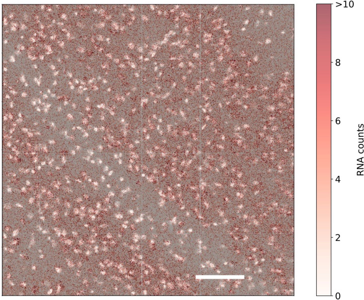
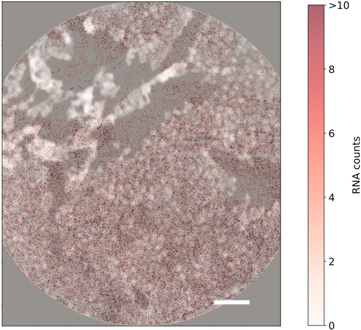
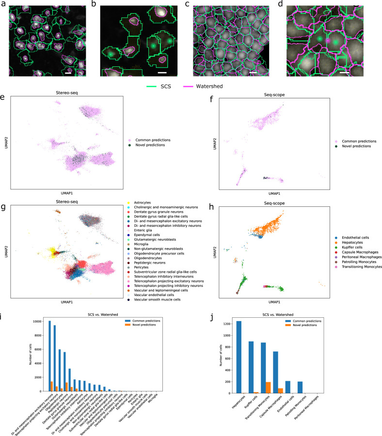
Spatial transcriptomics promises to greatly improve our understanding of tissue organization and cell-cell interactions. While most current platforms for spatial transcriptomics only offer multi-cellular resolution, with 10-15 cells per spot, recent technologies provide a much denser spot placement leading to sub-cellular resolution. A key challenge for these newer methods is cell segmentation and the assignment of spots to cells. Traditional image-based segmentation methods are limited and do not make full use of the information profiled by spatial transcrip-tomics. Here we present SCS, which combines imaging data with sequencing data to improve cell segmentation accuracy. SCS assigns spots to cells by adaptively learning the position of each spot relative to the center of its cell using a transformer neural network. SCS was tested on two new sub-cellular spatial transcriptomics technologies and outperformed traditional image-based segmentation methods. SCS achieved better accuracy, identified more cells, and provided more realistic cell size estimation. Sub-cellular analysis of RNAs using SCS spots assignments provides information on RNA localization and further supports the segmentation results.

Extended Data Figure 1

Extended Data Figure 2

Extended Data Figure 3

Extended Data Figure 4

Extended Data Figure 5

Figure 1:. Workflow of SCS.

a, Barcoded spots (cyan dots) that reside inside a cell nuclei (red masks) are first identified by segmenting the stained image. A transformer model is next trained on these spots and some background spots to predict the gradient direction (arrow) from each spot to the center of the cell to which it belongs and the probability that it is part of a cell (yellow arrow) or part of the extracellular matrix (purple arrow). The transformer model is then applied to all other spots. A gradient flow tracking algorithm is used to segment cells by grouping spots based on their gradient prediction. b, The transformer model predicts for each input spot the probabilities from this spot to its cell center for 16 predefined directions $(\widehat{d})$ and the probability that the spot is part of a cell (ŷ). For each spot (red dot), the transformer model aggregates information from its 50 nearest neighboring spots (cyan dots) by adaptively learning a weighting based on the spot expression (x) and relative positions (s). c, The structure of one transformer encoder layer, see “Methods” for details.

Figure 2:. Performance evaluation of SCS and comparisons with other methods.

a, The benchmark used for evaluating the performance and for comparison of differentsegmentation methods. The intersection region and respective difference (unique) regions between two segmentation are calculated for each cell. The segmentation is said to have higher accuracy if its unique cell region is better correlated with the intersection region. b, Comparison between SCS and the four other image segmentation methods using the correlation benchmark. Each cell used for evaluation contributes one point to the correlation presented in the boxplot. SCS achieved significantly higher segmentation accuracy than other methods on both datasets (Wilcoxon signed-rank tests, one-sided; for SCS vs. Watershed, N=17,811 cells on Stereo-seq, N=2,757 cells on Seq-scope; for SCS vs. Cellpose, N=13,310 cells on Stereo-seq, N=2,446 cells on Seq-scope; for SCS vs. DeepCell, N=26,916 cells on Stereo-seq, N=3,513 cells on Seq-scope, for SCS vs. StarDist, N=6,370 cells on Stereo-seq, N=2,635 cells on Seq-scope. Supplementary Note 3 for cell filtering criteria). c, Comparison of the sizes of cells segmented by SCS and other methods. SCS obtained segmented cells with larger cell diameters than all the other methods with significant differences on Stereo-seq (Kruskal-Wallis tests; for Stereo-seq, N=56,187 for SCS, N=52,004 for Watershed, N=50,020 for Cellpose, N=55,260 for DeepCell, N=55,364 for StarDist; for Seq-scope, N=4,456 for SCS, N=4,354 for Watershed, N=2,527 for Cellpose, N=4,157 for DeepCell, N=3,832 for StarDist). The red dashed lines show the expected cell diameters from the literature. d, The number of cells identified by the segmentation methods for the two datasets. b,c, Boxplots show medians (horizontal line in each box), interquartile ranges (boxes), 1.5 interquartile (whiskers), and remaining point individuals.

Figure 3:. Cell segmentation examples and the distributions of cells in low dimensional space.

a, SCS captured cytoplasm regions of cells in the nucleus staining and thus segmented cells with larger sizes. b, Example of segmentation results on the Stereo-seq dataset where Watershed missed three cells due to their low staining signal intensity while SCS identified them (green dots). c, Two segmentations show similar cell sizes but with disagreement on cell boundaries on the Seq-scope dataset. d, Segmentation example on the Seq-scope dataset where Watershed merged two cells as one cell (pink dot) due to their unclear boundary in the image while SCS successfully segmented them (green dots). e, UMAP projection of SCS segmented cells on the Stereo-seq dataset based on their expression profiles. Novel predictions (darker nodes) are mixed with cells identified using image segmentation. f, UMAP projection of SCS segmented cells on the Seq-scope dataset. g, Cell type annotation for the Stereo-seq dataset. h, Cell type annotation for the Seq-scope dataset. i, The number of novel cell predictions by SCS compared to Watershed vs. the number of cells that are commonly identified by SCS and Watershed in differentcell types for the Stereo-seq dataset. Cell types with more novel predictions are usually those with smaller nucleus sizes as shown in Supplementary Figure 4a. j, The same comparisons for the Seq-scope dataset. a-d, Experiments that generated the examples were independently repeated three times with similar results. Scale bars: 10 μm.

Figure 4:. Sub-cellular analysis using SCS.

a, Identification of genes whose RNAs are differentially localized. b, Volcano plot that shows quantitative changes in expression levels for genes between the nucleus and cytoplasm of SCS segmented cells for the Stereo-seq dataset. Genes with P-values < 0.01 and fold changes greater than 1.3 were identified from each group (t-tests, one-sided, the Benjamini-hochberg method was used to adjust P-values; N=31,763 nucleus regions, N=37,940 cytoplasm regions, subcellular regions with at least 100 genes were used for this analysis). Genes whose RNAs have been experimentally shown to reside in the nucleus or cytoplasm are colored accordingly. c, Volcano plot for the Seq-scope dataset. The top 100 genes with the smallest P-values were identified from each group (t-tests, one-sided, raw P-values are shown to avoid most of the P-values being corrected to the same value; N=2,779 nucleus regions, N=3,006 cytoplasm regions, regions with at least 100 genes were used for this analysis).

References

1. Li Dongshunyi, Ding Jun, and Bar-Joseph Ziv. Identifying signaling genes in spatial single-cell expression data. Bioinformatics, 37(7):968–975, 2021. - PMC - PubMed
1. Teng Haotian, Yuan Ye, and Bar-Joseph Ziv. Clustering spatial transcriptomics data. Bioinformatics, 38(4):997–1004, 2022. - PMC - PubMed
1. Ståhl Patrik L, Salmén Fredrik, Vickovic Sanja, Lundmark Anna, Navarro José Fernández, Magnusson Jens, Giacomello Stefania, Asp Michaela, Westholm Jakub O, Huss Mikael, et al. Visualization and analysis of gene expression in tissue sections by spatial transcriptomics. Science, 353(6294):78–82, 2016. - PubMed
1. Chen Ao, Liao Sha, Cheng Mengnan, Ma Kailong, Wu Liang, Lai Yiwei, Qiu Xiaojie, Yang Jin, Xu Jiangshan, Hao Shijie, et al. Spatiotemporal transcriptomic atlas of mouse organogenesis using dna nanoball-patterned arrays. Cell, 185(10):1777–1792, 2022. - PubMed
1. Cho Chun-Seok, Xi Jingyue, Si Yichen, Park Sung-Rye, Hsu Jer-En, Kim Myungjin, Jun Goo, Kang Hyun Min, and Lee Jun Hee. Microscopic examination of spatial transcriptome using seq-scope. Cell, 184(13):3559–3572, 2021. - PMC - PubMed
Publication types