AI-guided pipeline for protein-protein interaction drug discovery identifies a SARS-CoV-2 inhibitor

Abstract

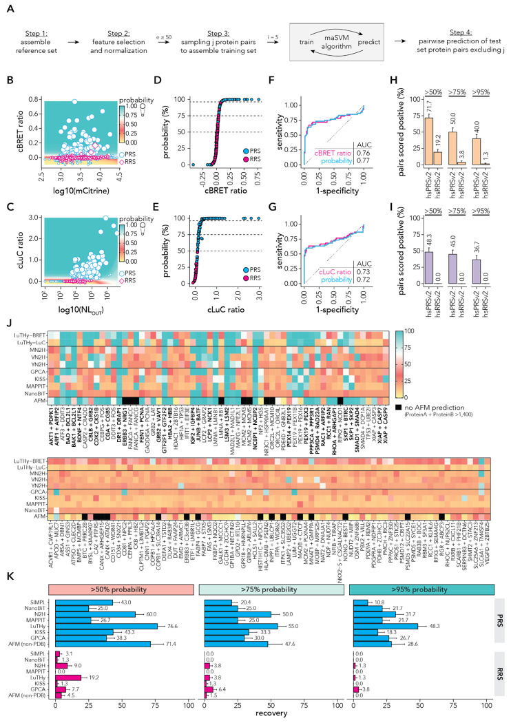
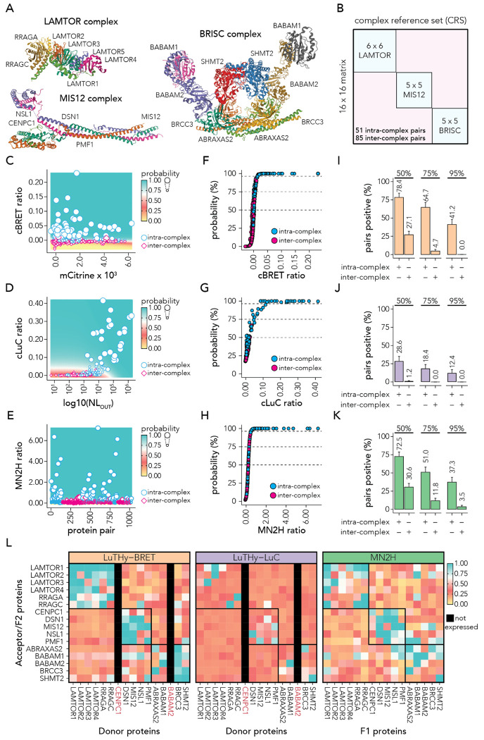
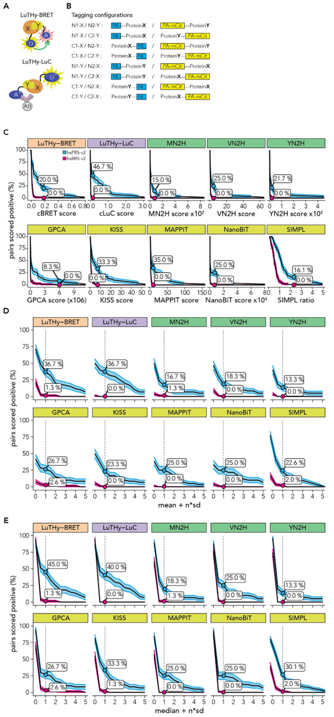
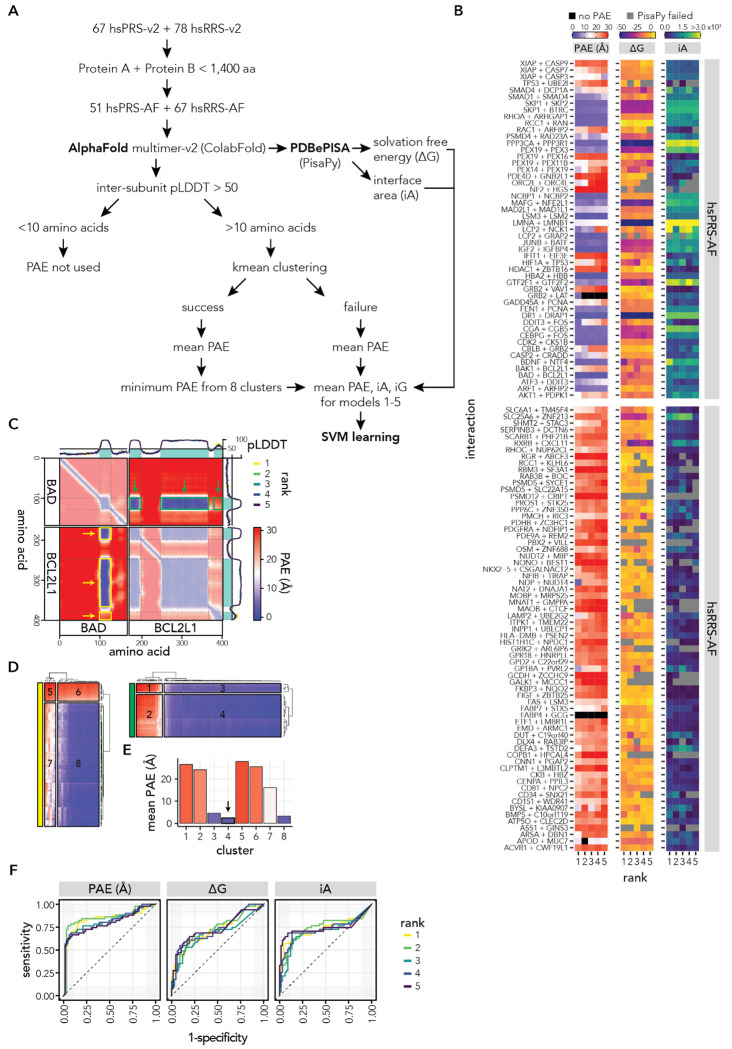
Protein-protein interactions (PPIs) offer great opportunities to expand the druggable proteome and therapeutically tackle various diseases, but remain challenging targets for drug discovery. Here, we provide a comprehensive pipeline that combines experimental and computational tools to identify and validate PPI targets and perform early-stage drug discovery. We have developed a machine learning approach that prioritizes interactions by analyzing quantitative data from binary PPI assays and AlphaFold-Multimer predictions. Using the quantitative assay LuTHy together with our machine learning algorithm, we identified high-confidence interactions among SARS-CoV-2 proteins for which we predicted three-dimensional structures using AlphaFold Multimer. We employed VirtualFlow to target the contact interface of the NSP10-NSP16 SARS-CoV-2 methyltransferase complex by ultra-large virtual drug screening. Thereby, we identified a compound that binds to NSP10 and inhibits its interaction with NSP16, while also disrupting the methyltransferase activity of the complex, and SARS-CoV-2 replication. Overall, this pipeline will help to prioritize PPI targets to accelerate the discovery of early-stage drug candidates targeting protein complexes and pathways.

Keywords: AlphaFold; SARS-CoV-2; VirtualFlow; machine learning; protein-protein interactions.

Figure 1.. Developing a maSVM algorithm to classify protein pairs from hsPRS-v2 and hsRRS-v2 using the LuTHy assay.

(A) Schematic overview of the maSVM learning algorithm. Step 1: assembly of reference set; Step 2: feature selection and RobustScaler normalization for reference and test set; Step 3: assembly of ‘e’ training sets (ensembles) by weighted sampling j protein pairs from the reference set to train ‘e≥50’ maSVM algorithms, where the training classifier labels are reclassified in ‘i=5’ iterations; Step 4: prediction of test set protein pairs excluding training set using the paired maSVM model. If classifier probabilities were not predicted for all test set protein pairs in ‘e=50’ ensembles, the maSVM algorithm was repeated from Step 3 assembling additional ‘e=10’ training sets excluding protein pairs from the training set that lack classifier probabilities. (B,C) Scatter plot showing (B) in-cell mCitrine expression (x-axis) against cBRET ratios (y-axis limited to ‘> −0.1’) or (C) luminescence after co-precipitation (NL_OUT) (x-axis) against cLuC ratios (y-axis) for all hsPRS-v2 (blue) and hsRRS-v2 (magenta) protein pairs from all eight tagging configurations. Average classifier probabilities from the 50 maSVM models are displayed as the size of the data points and as a colored grid in the background. (D,E) Scatter plot showing (D) cBRET ratios (x-axis) or (E) cLuC ratios (x-axis) against classifier probability (y-axis) for all hsPRS-v2 (blue) and hsRRS-v2 (magenta) protein pairs from all eight tagging configurations. (F,G) Receiver characteristic analysis comparing sensitivity and specificity between (F) cBRET ratios or (G) cLuC ratios and classifier probabilities. The calculated areas under the curve are displayed. (H,I) Bar plots showing the fraction of hsPRS-v2 and hsRRS-v2 protein pairs that scored above classifier probabilities of 50%, 75% or 95% by (H) LuTHy-BRET or (I) LuTHy-LuC. Only the highest classifier probability per tested tagging configuration is considered. (J) Heatmaps showing the highest classifier probabilities for the hsPRS-v2 (top) and hsRRS-v2 (bottom) protein pairs per tested tagging configuration. hsPRS-v2 interactions supported by structures or homologous structures are highlighted in bold. LuTHy and AFM data from this study; all other from Choi et al (Choi et al, 2019). (K) Bar plots showing the fraction of hsPRS-v2 and hsRRS-v2 protein pairs that scored above classifier probabilities of 50%, 75% or 95% for 10 binary PPI assay versions. Only the highest classifier probability per tested tagging configuration is considered. For AFM, the fraction of hsPRS-AF with no experimental structure or homologous structures (non-PDB) is shown (see Figure EV4D for recovery rate of all hsPRS-AF interactions). LuTHy and AFM data from this study; SIMPL from Yao et al (Yao et al, 2020); all other from Choi et al (Choi et al, 2019). Note that the SIMPL assay was benchmarked by Yao et al against 88 positive proteins pairs derived from the hsPRS-v1 (Venkatesan et al, 2009) and as a random reference set against “88 protein pairs with baits and preys selected from the PRS but used in combinations determined computationally to have low probability of interaction” (Yao et al, 2020).

Figure 2.. Validating the maSVM algorithm by mapping interactions within multiprotein complexes using the LuTHy and mN2H assays.

(A) Structures of the protein complexes analyzed in this study: LAMTOR (PDB: 6EHR), MIS12 (PDB: 5LSK), and BRISC (PDB: 6H3C). (B) Binary interaction approach to systematically map PPIs within distinct complexes. Every protein subunit from each complex was screened against every other one (all-by-all, 16x16 matrix). (C-E) Scatter plot showing (C) in-cell mCitrine expression (x-axis) against cBRET ratios (y-axis), (D) luminescence after co-precipitation (NL_OUT) (x-axis) against cLuC ratios (y-axis) or (E) the number of protein pairs (x-axis) against the mN2H ratios (y-axis) for all intra-complex (blue) and inter-complex (magenta) protein pairs from all eight tagging configurations. Average classifier probabilities from the 50 maSVM models are displayed as the size of the data points and as a colored grid in the background. (F-H) Scatter plot showing on the x-axis the (F) cBRET ratios , (G) cLuC ratios or (H) mN2H ratios against classifier probabilities (y-axis) for all intra-complex (blue) and inter-complex (magenta) protein pairs from all eight tagging configurations. (I-K) Bar plots showing the fraction of intra-complex and inter-complex protein pairs that scored above the classifier probabilities of 50%, 75% or 95% by (I) LuTHy-BRET, (J) LuTHy-LuC and (K) mN2H. Only the highest classifier probability per tested tagging configuration is considered. (L) Heatmaps showing the classifier probabilities for the Donor/F1 protein pairs (x-axis) against the Acceptor/F2 protein pairs (y-axis) for LuTHy-BRET (orange, left), LuTHy-LuC (purple, middle) and mN2H (green, right). Only the highest classifier probability per tested tagging configuration is shown. Not expressed constructs are filled black and protein names colored in red.

Figure 3.. Mapping binary interactions between SARS-CoV-2 proteins.

(A) Search space between SARS-CoV-2 proteins tested by LuTHy. (B) Strategy to classify screened SARS-CoV-2 protein pairs using the maSVM learning algorithm. The positive training set (PTS) was assembled from the hsPRS-v2 and the intra-complex protein pairs of the multiprotein complex set. The negative training set (NTS) was assembled from the hsRRS-v2 and the inter-complex protein pairs of the multiprotein complex set. The trained 50 models were used to predict the classifier probabilities of all LuTHy-BRET and LuTHy-LuC tested SARS-CoV-2 protein pairs. (C) Scatter plot showing in-cell mCitrine expression (x-axis) against cBRET ratios (y-axis) for SARS-CoV-2 (orange) protein pairs from all eight tagging configurations. Average classifier probability from the 50 maSVM models is displayed as the size of the data points and as a colored grid in the background. (D) Scatter plot showing cBRET ratios (x-axis) against classifier probability (y-axis) for all SARS-CoV-2 (orange) protein pairs from all eight tagging configurations for LuTHy-BRET. (E) Scatter plot showing luminescence after co-precipitation (NL_OUT) (x-axis) against cLuC ratios (y-axis) for SARS-CoV-2 (orange) protein pairs from all eight tagging configurations. Average classifier probability from the 50 maSVM models is displayed as the size of the data points and as a colored grid in the background. (F) Scatter plot showing cLuC ratios (x-axis) against classifier probability (y-axis) for all SARS-CoV-2 (orange) protein pairs from all eight tagging configurations for LuTHy-LuC. The number of protein pairs with classifier probabilities of >50%, >75% and >95% are indicated. (G,H) Binary heatmaps showing SARS-CoV-2 protein pairs with >95% classifier probability detected with (G) LuTHy-BRET and (H) LuTHy-LuC. Only the highest classifier probability per tested tagging configuration is shown.

Figure 4.. Predicting the NSP10-NSP16 PPI complex with AFM to target the interaction interface by ultra-large virtual drug screening.

(A) Heatmap showing the predicted alignment error (PAE) of the AlphaFold-Multimer predicted NSP10-NSP16 complex for the rank 1 model. The intra-molecular PAEs are shown with 50% opacity. The predicted local distance difference test (pLDDT) for all five predicted models (rank 1-5) are shown as line graphs on top and on the right of the heatmap. The area with pLDDT scores >50 is highlighted in teal. (B) The five models of the AlphaFold-Multimer predicted NSP10-NSP16 complex and the published crystal structure (PDB: 6W4H) are shown. Structures were overlaid using the ‘matchmaker’ tool of ChimeraX. (C) Scatter plot showing for each amino acid (x-axis) the solvation free energy (ΔG, y-axis, fill color) upon formation of the interface, in kcal/M, as determined by PDBePISA. Dots represent the average ΔG for the five predicted models and error bars correspond to the standard deviation. Lysine 93 of NSP10 is indicated. (D) Zoom-in into the NSP10-NSP16 complex showing the contacts of NSPIOs Lysine 93. (E) LuTHy-BRET donor saturation assay, where constant amounts of NSP10-NL wt or K93E are co-expressed with increasing amounts of mCitrine-NSP16. Non-linear regression was fitted through the data using the One-Site – Total’ equation of GraphPad Prism. (F) Docking box on the NSP10 structure (PDB: 6W4H) used for the ultra-large virtual screen. (G) Schematic overview of the workflow of the virtual docking screen using VirtualFlow. (H) Docking scores of the top 100 molecules identified that target NSP10.

Figure 5.. Compound 459 inhibits the NSP10-NSP16 interaction and reduces SARS-CoV-2 replication.

(A) Schematic overview of the NSP10-NSP16 methyltransferase (MTase) assay. (B) Heatmap showing the result of the MTase activity of the NSP10-NSP16 complex in the absence or presence of 100 μM of the top 15 compounds. Statistical significance was calculated with a kruskal-wallis test (p-value = 9.7e-5, chi-squared = 47.656, df = 17, n = 3), followed by a post-hoc Dunn test and adjusted p-values are shown. (C) Compound 459 docked onto the NSP10 structure (PDB: 6W4H). (D) Chemical structure of compound 459. (E) Assay principle of the microscale thermophoresis (MST) assay. The fluorescence intensity change of the labeled molecule (purple) after temperature change induced by an infrared laser (red) is measured. The binding of a non-fluorescent molecule (blue) can influence the movement of the labeled molecule. (F) Representative MST traces of labeled NSP10 and different concentrations of unlabeled compound 459. The bound fraction is calculated from the ratio between the fluorescence after heating (F₁) and before heating (F₀). (G) Scatter plot showing the 459 concentrations (x-axis) against the fraction of 459 bound to NSP10 (y-axis). Non-linear regression was fitted through the data using the One-Site – Total’ equation of GraphPad Prism (n = 3). (H) Scatter plot showing the 459 concentrations (x-axis) against the normalized BRET ratio (nBRET ratio) for the interaction between NSP10-NL and mCit-NSP16. Non-linear regression was fitted through the data using the ‘log(inhibitor) vs. response – Variable slope (four parameters)’ equation of GraphPad Prism (n = 4). (I) Scatter plot showing the 459 concentrations (x-axis) against the relative luminescence measured from icSARS-CoV-2-nanoluciferase in HEK293-ACE2 cells. Non-linear regression was fitted through the data using the ‘log(inhibitor) vs. normalized response’ equation of GraphPad Prism (n = 9). (J) Bar plot showing the relative luminescence measured from icSARS-CoV-2-nanoluciferase in HEK293-ACE2 cells upon incubation with 0, 25, 50 or 100 μM of compound 459 together with 2.5 μM AZ1 or without AZ1 (0.0 μM). Statistical significance was calculated in GraphPad Prism by a Two-way Anova’, where each cell mean was compared to the other cell mean in that row using ‘Bonferroni’s multiple comparisons test’ (n = 3; source of variation: 57.91% 459 concentration, p<0.0001; 28.33% AZ1 concentration, p<0.0001; 11.40% 459/AZ1 interaction, p<0.0001).

Figure EV1 (related to Figure 1).. Effect of different scoring approaches on recovery rates.

(A) Schematic overview of the LuTHy-BRET and LuTHy-LuC assays. X: Protein X, Y: Protein Y, D: NanoLuc donor, A: mCitrine acceptor, AB: antibody. (B) With the LuTHy assay, each protein pairX-Y can be tested in eight possible configurations (N-vs. C-terminal fusion for each protein), and proteins can be swapped from one tag to the other resulting in 16 quantitative scores for each protein pair, i.e. eight for LuTHy-BRET and eight for LuTHy-LuC. (C) Line plots showing the fraction of protein pairs that scored positive (y-axis) dependent on the quantitative interaction scores (x-axis) for 10 binary PPI assay versions. For each tested protein pair, the tagging configuration with the highest interaction score is used. For LuTHy all eight tagging configurations were tested, whereas for MN2H, VN2H, YN2H, GPCA, NanoBi four and for KISS, MAPPIT and SIMPL two tagging configurations were tested. Recovery rates at maximum specificity, i.e. where none of the protein pairs in the RRS scored positive (0%), are indicated. Note that in Choi et al. (Choi et al, 2019) recovery rates at maximum specificity were calculated by using distinct cut-offs for each tagging configuration. (D) Line plots showing the fraction of protein pairs that scored positive (y-axis) dependent on the distribution of interaction scores, i.e. the mean of all interaction scores + n*(sd) (x-axis) for 10 binary PPI assay versions. Recovery rates at mean + 1 standard deviation are indicated (E) Line plots showing the fraction of protein pairs that scored positive (y-axis) dependent on the distribution of interaction scores, i.e. the median of all interaction scores + n*(sd) (x-axis) for 10 binary PPI assays. Recovery rates at median + 1 standard deviation are indicated. LuTHy data from this study; SIMPL from Yao et al (Yao et al, 2020); all other from Choi et al (Choi et al, 2019). Note that the SIMPL assay was benchmarked by Yao et al (Yao et al, 2020) against 88 positive proteins pairs derived from the hsPRS-v1 (Venkatesan et al, 2009) and as a random reference set against “88 protein pairs with baits and preys selected from the PRS but used in combinations determined computationally to have low probability of interaction” (Yao et al, 2020).

Figure EV2 (related to Figure 1).. Establishment and performance of the maSVM algorithm.

(A) Schematic overview to evaluate the performance when using either a fixed cutoff or the maSVM learning algorithm, by separating the hsPRS-v2 and hsRRS-v2 randomly into a training (70%) and a test (30%) set in k = 20 iterations. (B,C) Boxplots showing the fraction of protein pairs that scored positive in the training and the test sets (from A) using a fixed-cutoff at a maximum specificity, i.e. where none of the interactions of the RRS of the training set scored positive by (B) LuTHy-BRET or (C) LuTHy-LuC. Each dot represents the recovery rates from one of the 20 iterations. Numbers above boxplot indicate the mean and in brackets the standard deviation. The cutoffs used to determine the fraction of protein pairs that scored positive in the test were used from each respective training set k at 0% RRS. (D,E) Representative scatter plot for the first SVM model for the LuTHy-BRET showing in-cell mCitrine expression (x-axis) against cBRET ratios (y-axis) from the (D) first training set (k = 1), from which in the first ensemble (e = 1) 90 protein pairs (j) were randomly sampled and reclassified in 5 iterations (i = 5). (E) Scatter plot for the first test set (k = 1), that contains 336 protein pair configurations. The classification models from the first SVM model (from D) are visualized in (D,E) as different colors (negativ = yellow; positive = teal) that are separated by the support vector. The known classification of the protein pairs of the train and test set are indicated by color (blue = PRS; magenta = RRS). (F,G) Representative scatter plot for the first SVM model for the LuTHy-LuC showing luminescence after co-precipitation (x-axis) against cLuC ratios (y-axis) from the (F) first training set (k = 1), from which in the first ensemble (e = 1) 90 protein pairs (j) were randomly sampled and reclassified in 5 iterations (i = 5). (G) Scatter plot for the first test set (k = 1), that contains 336 protein pair configurations. The classification models from the first SVM model (from F) are visualized in (F,G) as different colors (negativ = yellow; positive = teal) that are separated by the support vector. The known classification of the protein pairs of the train and test set are indicated by color (blue = PRS; magenta = RRS). (H,I) Scatter plot showing (H) cBRET ratios (x-axis) or (I) cLuC ratios (x-axis) against the average classifier probability (y-axis) for all hsPRS-v2 (blue) and hsRRS-v2 (magenta) protein pairs from all eight tagging configurations. The classifier probability was averaged over the twenty assembled training and test sets (k) and standard deviations are indicated. (J-K) Box plots showing the fraction of hsPRS-v2 and hsRRS-v2 protein pairs that scored above classifier probabilities of 50%, 75% or 95% by (J) LuTHy-BRET and (K) LuTHy-LuC. Each dot represents the results from one assembled test and training set (k). Numbers above boxplot indicate the mean and in brackets the standard deviation. (L) Scatter plots for eight quantitative PPI assay variants showing the number of protein pairs (x-axis) against their respective interaction scores (y-axis) for hsPRS-v2 (blue) and hsRRS-v2 (magenta) protein pairs. Average classifier probability from the 50 maSVM models is displayed as the size of the data points and as a colored grid in the background. The maSVM algorithm for the SIMPL assay was trained on the SIMPL interaction score (mean SIMPL, x-axis) and the ratio between SIMPL interaction score and bait expression (mean ratio, y-axis) using the published data from Yao et al (Yao et al, 2020). Note that the SIMPL assay was benchmarked against 88 positive proteins pairs derived from the hsPRS-v1 (Venkatesan et al, 2009) and as a random reference set against “88 protein pairs with baits and preys selected from the PRS but used in combinations determined computationally to have low probability of interaction” (Yao et al, 2020). Data for all other assays is from Choi et al (Choi et al, 2019).

Figure EV3 (related to Figure 1):. Benchmarking AFM using well-established positive and random reference sets.

(A) Schematic overview of AlphaFold-multimer (AFM) benchmarking. First, the hsPRS-v2 and hsRRS-v2 were filtered for protein pairs with less than 1,400 amino acids combined, resulting in 51 positive reference set pairs (hsPRS-AF) and 67 random reference set pairs (hsRRS-AF). For these 118 protein pairs, five structural models were predicted using ColabFold through the AFM algorithm (590 total structures). Following, PAE and pLDDT values were extracted from the AFM predicted structures, and inter-subunit amino acids were filtered for pLDDT >50. If >10 inter-subunit amino acids remained, PAE values were k-means clustered. If clustering failed, the mean PAE of the unclustered amino acids was calculated, else the average PAE of the eight clusters were calculated and the minimum PAE selected as the amino acid region with the minimal distance between the two proteins. In addition, PDBePISA was used to determine the solvation free energy (ΔG) and the area (iA) of the interface region (Python script PisaPy was used for batch analysis) for 521 of the 590 structures. For the remaining 69 structures PDBePISA could not identify an interface. Next, the average PAE, iA and ΔG were calculated for the five predicted structural models of the 51 hsPRS-AF and 67 hsRRS-AF protein pairs. Finally, a multi-adaptive maSVM learning algorithm was trained on the PAE and iA features of the hsPRS-AF and hsRRS-AF as outlined in Figure 1A. The 50 trained models were ultimately used to predict the classifier probability of the CoV-2-AF structures in Figure EV7B-E. (B) Heatmap of the PAEs, ΔGs and iAs for protein pairs of the hsPRS-AF and hsRRS-AF. Shown are the minimum PAE values after kmeans clustering. If <10 amino acids had pLDDT >50 the PAE values were not used and shown in black. Protein pairs where no interaction interface was detected by PDBePISA are shown in gray. (C) Representative example for the kmeans clustering strategy of AFM reported PAE values. Heatmap shows the PAEs for the protein pair BAD+BCL2L1 (hsPRS-AF) rank 1 model. The intra-molecular PAEs are shown with 50% opacity. The predicted local distance difference test (pLDDT) for all five predicted models (rank 1-5) are shown as line graphs on top and on the right of the heatmap. The area with pLDDT scores >50 is highlighted in teal. Inter-molecular regions with pLDDT >50 that were used for kmeans clustering are highlighted with green (BAD>BCL2L1 interface) and yellow (BCL2L1>BAD interface) boxes that are also indicated with arrows. (D) Clustering results of green and yellow regions highlighted in panel C. Cluster numbers are indicated. (E) Average PAE values for the eight clusters from panels C and D. The arrow indicates the cluster with the lowest average PAE value. (F) Receiver characteristic analysis comparing sensitivity and specificity between the five ranked structural models for PAE, ΔG and iA of the hsPRS-AF and hsRRS-AF.

Figure EV4 (related to Figure 1):. Training a maSVM algorithm to classify AFM predicted structures.

(A) Scatter plot showing PAE (x-axis) against interface area (y-axis) for all hsPRS-AF (blue) and hsRRS-AF (magenta) protein pairs. Average classifier probability from the 50 maSVM models is displayed as the size of the data points and as a colored grid in the background. (B) Scatter plots showing PAE (x-axis, left panel) or interface area (x-axis, right panel) against classifier probability (y-axis) for all hsPRS-AF (blue) and hsRRS-AF (magenta) protein pairs. (C) Bar plots showing the fraction of hsPRS-AF and hsRRS-AF protein pairs that scored above classifier probabilities of 50%, 75% and 95%. (D) Bar plots showing the fraction of hsPRS-AF and hsRRS-AF interactions with structures deposited in PDB that scored above classifier probabilities of 50%, 75% and 95% by AlphaFold-Multimer (i) and the fraction of hsPRS-v2 and hsRRS-v2 interactions with structures deposited in PDB that scored above classifier probabilities of 50%, 75% or 95% by LuTHy (ii) or the union of five other binary assays (iii), N2H (MN2H, VN2H, YN2H), GPCA, KISS, MAPPIT and NanoBiT. Data for the SIMPL assay was excluded for this analysis due to the different composition of the reference sets.

Figure EV5 (related to Figure 2).. Construct-specific robust scaler normalization for mapping multiprotein complexes.

(A-H) Boxplots of assay specific interaction scores before and after robust scaler normalization for the multiprotein complex proteins in all tagging configurations of donor and acceptor constructs. Boxplots display the constructs’ median, lower and upper hinges the 25^th and 75^th percentiles, lower and upper whiskers extending from the hinges with 1.5x the inter-quartile range and outlier points beyond the end of the whiskers. The thick horizontal line indicates the median interaction score over all constructs of the multiprotein complex set and the dashed lines the respective IQR of the 25^th and 75^th quartiles. Note that the horizontal lines always refer to the median and IQR before normalization and that the range of the y-axis is limited to visualize all boxplots as well as the median and IQR, but high scoring protein pairs (outliers) are hidden. (A) cBRET ratios for donor constructs before (top) and after (bottom) robust scaler normalization. (B) cBRET ratios for acceptor constructs before (top) and after (bottom) robust scaler normalization. (C) cLuC ratios for donor constructs before (top) and after (bottom) robust scaler normalization. (D) cLuC ratios for acceptor constructs before (top) and after (bottom) robust scaler normalization. (E) Luminescence after co-precipitation (NL_OUT) for donor constructs before (top) and after (bottom) robust scaler normalization. (F) Luminescence after co-precipitation (NL_OUT) for acceptor constructs before (top) and after (bottom) robust scaler normalization. (G) mN2H ratios for F1 constructs before (top) and after (bottom) robust scaler normalization. (H) mN2H ratios for F2 constructs before (top) and after (bottom) robust scaler normalization.

Figure EV6 (related to Figure 3).. Construct-specific robust scaler normalization for SARS-CoV-2 binary PPI mapping.

(A-F) Boxplots of LuTHy-BRET and LuTHy-LuC interaction scores before and after robust scaler normalization for the SARS-CoV-2 proteins in all tagging configurations of donor and acceptor constructs. Boxplots display the constructs’ median, lower and upper hinges the 25^th and 75^th percentiles, lower and upper whiskers extending from the hinges with 1.5x the inter-quartile range and outlier points beyond the end of the whiskers. The thick horizontal line indicates the median interaction score over all constructs of the training (hsPRS-v2, hsRRS-v2, multiprotein complex) and test set (SARS-CoV-2) and the dashed lines the respective IQR of the 25^th and 75^th quartiles. Note that the horizontal lines always refer to the median and IQR before normalization and that the range of the y-axis is limited to visualize all boxplots as well as the median and IQR, but high scoring protein paris (outliers) are hidden. (A) cBRET ratios for donor constructs before (top) and after (bottom) robust scaler normalization. (B) cBRET ratios for acceptor constructs before (top) and after (bottom) robust scaler normalization. (C) cLuC ratios for donor constructs before (top) and after (bottom) robust scaler normalization. (D) cLuC ratios for acceptor constructs before (top) and after (bottom) robust scaler normalization. (E) Luminescence after co-precipitation (NL_OUT) for donor constructs before (top) and after (bottom) robust scaler normalization. (F) Luminescence after co-precipitation (NL_OUT) for acceptor constructs before (top) and after (bottom) robust scaler normalization.

Figure EV7 (related to Figure 5 and Figure EV5).. Predicting SARS-CoV-2 protein complex structures using AlphaFold Multimer.

(A) Venn diagrams showing the overlap between interactions recovered by LuTHy at >50%, >75% and >95% probabilities and interactions deposited in the IntAct database (Orchard et al, 2014) (B) Boxplots showing predicted alignment error (PAE), solvation free energy (ΔG) and interface area (iA) from AlphaFold-Multimer (AFM) predicted SARS-CoV-2-AF structures. Boxplots display the median, lower and upper hinges the 25^th and 75^th percentiles and lower and upper whiskers extending from the hinges with 1.5x the inter-quartile range. Each dot represents one predicted structural model. (C) Scatter plot showing PAE (x-axis) against interface area (y-axis) for all SARS-CoV-2-AF (orange) protein pairs. Average classifier probability predicted by the 50 maSVM models trained by the hsPRS-AF and hsRRS-AF set (see Figure EV4A), is displayed as the size of the data points. Each point in the colored grid in the background displays the average classifier probabilities from the 50 maSVM models. (D) Scatter plots showing PAE (x-axis, left panel) or interface area (x-axis, right panel) against classifier probability (y-axis) for all SARS-CoV-2-AF (orange) protein pairs. (E) Bar plots showing the fraction of SARS-CoV-2-AF protein pairs that scored above classifier probabilities of 50%, 75% and 95%. (F) Heatmap showing the classifier probabilities for the AFM predicted protein pair structures of the SARS-CoV-2-AF protein pairs. (G) Scatter plot showing the average ΔG (x-axis) from the five predicted structural SARS-CoV-2-AF models against the LuTHy-BRET determined binding strengths (BRET₅₀, see Figure EV8A). Only SARS-CoV-2 predicted AFM structures with classifier probabilities of >75% are shown and the respective classifier probabilities are indicated by the fill color of the data points. A linear regression fit through the data is shown and the Spearman correlation coefficient (R) and p-value are indicated. (H) Barplot showing the fraction of AFM predicted structures with 0-75%, 75-95% and >95% classification probability that have an experimentally reported structure deposited to the PDB (Berman et al, 2000) database. (I,J) Luminescence (I) and fluorescence (J) values from LuTHy-BRET donor saturation experiment, where constant amounts of NSP10-NL wt or K93E are co-expressed with increasing amounts of mCitrine-NSP16.

Figure EV8 (related to Figure 4 and Figure EV7).. LuTHy-BRET binding strengths for CoV-2-AF protein complexes.

(A,B) Scatter plots showing LuTHy-BRET donor saturation curves with the acceptor to donor ratio (x-axis) plotted against the BRET ratio (y-axis) for 16 CoV-2-AF protein pairs with classifier probabilities >75%. A non-linear regression fit was performed using the ‘One site – Total and nonspecific binding’ in GraphPad Prism, using the results from the ‘NL-X/X-NL + mCit’ protein pair to subtract nonspecific binding in order to calculate the acceptor to donor ratios at half-maximal BRET ratios (BRET₅₀). BRET₅₀ values for protein pairs in (A) were used in Figure EV7F. (B) For the homodimer between NSP4-NSP4 the calculation of a BRET₅₀ failed due to the linear relation between acceptor : donor and the BRET ratio. The linear relation can be the result of an unspecific binding between the two proteins or because of a higher order oligomerization of the protein.

References

1. Abdelaal T, Michielsen L, Cats D, Hoogduin D, Mei H, Reinders MJT & Mahfouz A (2019) A comparison of automatic cell identification methods for single-cell RNA sequencing data. Genome Biol 20: 194. - PMC - PubMed
1. Alhossary A, Handoko SD, Mu Y & Kwoh C-K (2015) Fast, accurate, and reliable molecular docking with QuickVina 2. Bioinformatics 31: 2214–2216 - PubMed
1. Araujo MEG de, Naschberger A, Fürnrohr BG, Stasyk T, Dunzendorfer-Matt T, Lechner S, Welti S, Kremser L, Shivalingaiah G, Offterdinger M, et al. (2017) Crystal structure of the human lysosomal mTORC1 scaffold complex and its impact on signaling. Science 358: 377–381 - PubMed
1. Baek M, DiMaio F, Anishchenko I, Dauparas J, Ovchinnikov S, Lee GR, Wang J, Cong Q, Kinch LN, Schaeffer RD, et al. (2021) Accurate prediction of protein structures and interactions using a three-track neural network. Science: eabj8754 - PMC - PubMed
1. Berman HM, Westbrook J, Feng Z, Gilliland G, Bhat TN, Weissig H, Shindyalov IN & Bourne PE (2000) The Protein Data Bank. Nucleic Acids Res 28: 235–242 - PMC - PubMed
Publication types