Linear fine-tuning: a linear transformation based transfer strategy for deep MRI reconstruction

Abstract

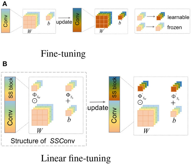
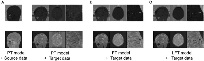
Introduction: Fine-tuning (FT) is a generally adopted transfer learning method for deep learning-based magnetic resonance imaging (MRI) reconstruction. In this approach, the reconstruction model is initialized with pre-trained weights derived from a source domain with ample data and subsequently updated with limited data from the target domain. However, the direct full-weight update strategy can pose the risk of "catastrophic forgetting" and overfitting, hindering its effectiveness. The goal of this study is to develop a zero-weight update transfer strategy to preserve pre-trained generic knowledge and reduce overfitting.

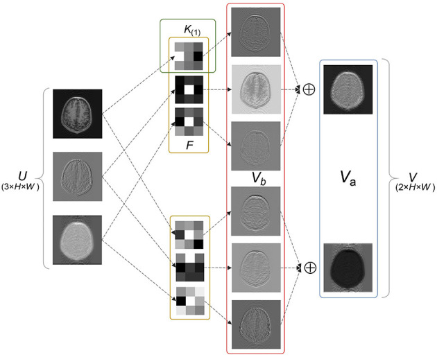
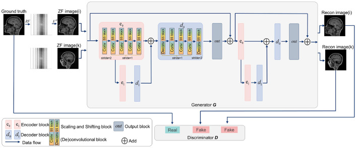
Methods: Based on the commonality between the source and target domains, we assume a linear transformation relationship of the optimal model weights from the source domain to the target domain. Accordingly, we propose a novel transfer strategy, linear fine-tuning (LFT), which introduces scaling and shifting (SS) factors into the pre-trained model. In contrast to FT, LFT only updates SS factors in the transfer phase, while the pre-trained weights remain fixed.

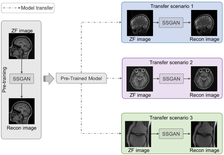
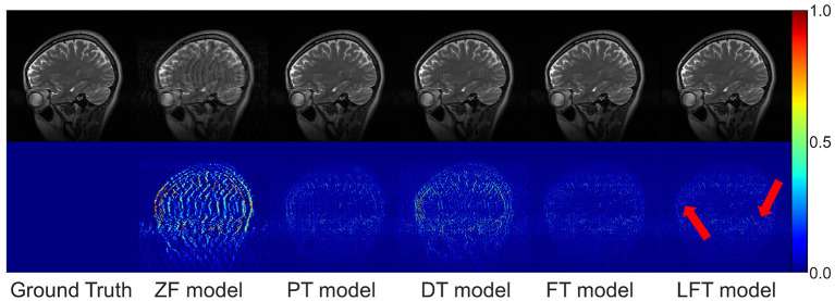
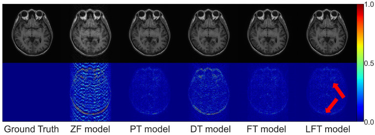
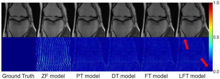
Results: To evaluate the proposed LFT, we designed three different transfer scenarios and conducted a comparative analysis of FT, LFT, and other methods at various sampling rates and data volumes. In the transfer scenario between different contrasts, LFT outperforms typical transfer strategies at various sampling rates and considerably reduces artifacts on reconstructed images. In transfer scenarios between different slice directions or anatomical structures, LFT surpasses the FT method, particularly when the target domain contains a decreasing number of training images, with a maximum improvement of up to 2.06 dB (5.89%) in peak signal-to-noise ratio.

Discussion: The LFT strategy shows great potential to address the issues of "catastrophic forgetting" and overfitting in transfer scenarios for MRI reconstruction, while reducing the reliance on the amount of data in the target domain. Linear fine-tuning is expected to shorten the development cycle of reconstruction models for adapting complicated clinical scenarios, thereby enhancing the clinical applicability of deep MRI reconstruction.

Keywords: deep learning; fine-tuning; magnetic resonance imaging reconstruction; transfer learning; transfer strategy.

Figure 1

Exemplary basic and advanced features. V_b and V_a represent the outputs of each kernel and each filter, respectively. V_a shows two types of advanced features including in-contour artifacts (top) and out-of-contour artifacts (bottom).

Figure 2

Visualization of the difference between FT and LFT in the transfer phase. Taking a 3 × 3 filter as an example with four channels, the structure of SSConv is composed of SS block and regular convolution. The 3 × 3 and 1 × 1 squares represent the weight W and bias b of the kernel, respectively, and different colors in them symbolize different channels. (A) FT updates all the pre-trained W and b. (B) The propose LFT optimizes the scaling factor Φ_SW and shifting factor Φ_Sb only.

Figure 3

Overview of the SSGAN architecture. The generator G of SSGAN is composed of two residual U-net with 2 encoder (pink box) and 2 decoder (blue box) blocks. The architecture of the discriminator D is the same as the encoding path of G. The inputs of G are the ZF image (i) and ZF image (k), which come from different collections.

Figure 4

Three transfer scenarios of the pre-trained SSGAN. The gray part shows SSGAN was pre-trained on the IXI dataset, then transferred to reconstruct images with different contrasts (blue part, scenario 1: T1-weighted to T2-weighted), slicing directions (purple part, scenario 2: axial planes to sagittal planes), and anatomical structures (green part, scenario 3: brain to knee).

Figure 5

Comparison of advanced features extracted by filters of the same channel in four cases: advanced features obtained by (A) feeding the source data into the PT model; (B) feeding the target data into the PT model; (C) feeding the target data into the FT model; (D) feeding the target data into the LFT model. Source data is from IXI dataset, while target data are from private sagittal brain dataset I, private axial brain dataset II, and FastMRI knee dataset.

Figure 6

Typical reconstructions for sagittal T2-weighted brains from private dataset I by different methods. The last three models trained with 160 images at 50% sampling rate. From left to right are the results of: ground truth, zero-filled model, pre-trained model, directly trained model, fine-tuning model, and linear fine-tuning model, as well as their 10× magnified error maps.

Figure 7

Typical reconstructions for axial T1-weighted brain images from private dataset II by different models (the last three networks trained with 200 images at 50% sampling rate). From left to right are the results of: ground truth, zero-filled model, pre-trained model, directly trained model, fine-tuning model, and linear fine-tuning model.

Figure 8

Typical reconstructions for knee images from FastMRI dataset by different networks (the last three networks trained with 200 images at 50% sampling rate). From left to right are the results of: ground truth, zero-filled model, pre-trained model, directly trained model, fine-tuning model, and linear fine-tuning model.