Remapping in a recurrent neural network model of navigation and context inference

Abstract

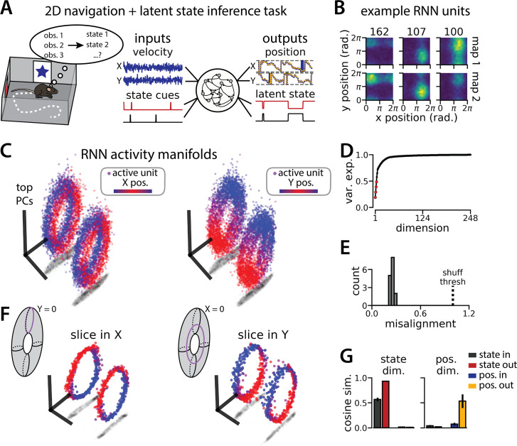
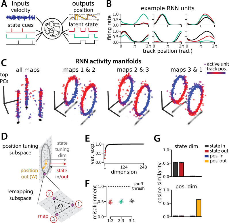
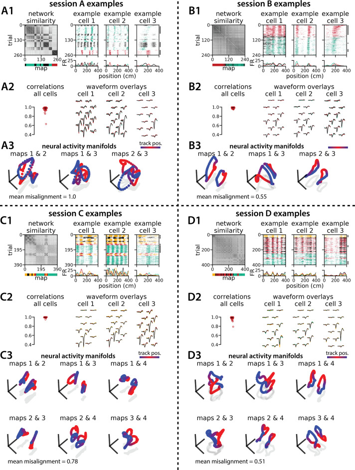
Neurons in navigational brain regions provide information about position, orientation, and speed relative to environmental landmarks. These cells also change their firing patterns ('remap') in response to changing contextual factors such as environmental cues, task conditions, and behavioral states, which influence neural activity throughout the brain. How can navigational circuits preserve their local computations while responding to global context changes? To investigate this question, we trained recurrent neural network models to track position in simple environments while at the same time reporting transiently-cued context changes. We show that these combined task constraints (navigation and context inference) produce activity patterns that are qualitatively similar to population-wide remapping in the entorhinal cortex, a navigational brain region. Furthermore, the models identify a solution that generalizes to more complex navigation and inference tasks. We thus provide a simple, general, and experimentally-grounded model of remapping as one neural circuit performing both navigation and context inference.

Keywords: Recurrent neural network models; attractor manifolds; dynamic coding; latent state; medial entorhinal cortex; mouse; navigation; neuroscience.

Figure 1.. Recurrent neural network (RNN) models and biological neural circuits remap between aligned spatial maps of a single 1D environment.

(A–D) are modified from Low et al., 2021. (A) Schematized task. Mice navigated virtual 1D circular-linear tracks with unchanging environmental cues and task conditions. Neuropixels recording probes were inserted during navigation. (B) Schematic: slower running speeds correlated with the remapping of neural firing patterns. (C, left) An example medial entorhinal cortex neuron switches between two maps of the same track (top, spikes by trial and track position; bottom, average firing rate by position across trials from each map; red, map 1; black, map 2). (C, right/top) Correlation between the spatial firing patterns of all co-recorded neurons for each pair of trials in the same example session (dark gray, high correlation; light gray, low correlation). The population-wide activity is alternating between two stable maps across blocks of trials. (C, right/bottom) K-means clustering of spatial firing patterns results in a map assignment for each trial. (D) Principal Components Analysis (PCA) projection of the manifolds associated with the two maps (color bar indicates track position). (E) RNN models were trained on a simultaneous 1D navigation (velocity signal, top) and latent state inference (transient, binary latent state signal, bottom) task. (F) Example showing high prediction performance for the position (top) and latent state (bottom). (G) As in (C), but for RNN units and network activity. Map is the predominant latent state on each trial. (H) Example PCA projection of the moment-to-moment RNN activity (colormap indicates track position). (I) Total variance explained by the principal components for network-wide activity across maps (top three principal components, red points). (J) Normalized manifold misalignment scores across models (0, perfectly aligned; 1, p=0.25 of shuffle). (K) Cosine similarity between the latent state and position input and output weights onto the remap dimension (left) and the position subspace (right) (error bars, sem; N = 15 models).

Figure 1—figure supplement 1.. Single recurrent neural network (RNN) units remap heterogeneously.

(A) Absolute fold change in peak firing rate versus spatial dissimilarity across latent state changes for all units from 2-map RNN models (points, single units; histograms, density distributions for each variable). Median change in peak firing rate (horizontal red dashes)=1.9 fold; 95^th percentile (horizontal gold dashes)=threefold. Median spatial dissimilarity (vertical red dashes)=0.025; 95^th percentile (vertical gold dashes)=0.21. (B) Modified from Low et al., 2021. As in (A) but for biological neurons from 2-map sessions. Median change in peak firing rate (horizontal red dashes)=1.28 fold. Median spatial dissimilarity (vertical red dashes)=0.031; 95^th percentile (vertical gold dashes)=0.22.

Figure 1—figure supplement 2.. Recurrent neural network (RNN) geometry is interpretable.

(A) Schematic showing the relative orientation of the position output weights and the context input and output weights to the position and state tuning subspaces. (B) Reproduced from Figure 1K. (C–D) Schematic to interpret why the position input weights are orthogonal to the position-uning subspace. These schematics illustrate how a single velocity input (blue arrows) updates the position estimate (yellow to red points) from a given starting position (blue points). (C, not observed) Velocity input lies in the position tuning subspace (gray plane). Note that the same velocity input pushes the network clockwise or counterclockwise along the ring depending on the circular position. (D, observed) Velocity input is orthogonal to the position tuning subspace and pushes neural activity out of the subspace. (E) Schematic of possible flow fields in each of three planes (numbers correspond to planes in C and D). We conjecture that these dynamics would enable a given orthogonal velocity input to nonlinearly update the position estimate, resulting in the correct translation around the ring regardless of starting position (as in D).

Figure 2.. The ring attractors are more aligned than strictly required by the task.

(A) Schematic illustrating how the two attractor rings could be misaligned in the nullspace of the position output weights (left) while still allowing linear position decoding (right) (color map, track position; solid arrows, remapping vectors; dashed arrow, projection onto the position subspace). (B) Schematic illustrating perfect manifold alignment (colors as in A) (C) Normalized difference between the true remapping vectors for all position bins and all models and the ideal remapping vector (dashed line, p=0.025 of shuffle; n=50 position bins, 15 models). (D) Dimensionality of the remapping vectors for an example model. (Right) Total variance explained by the principal components for the remapping vectors (red points, top two PCs). (Left) Relative variance is explained by the remapping vectors (red) and the position rings (blue) (1=total network variance). (E) The remapping vectors vary smoothly over the position. (Right) Projection of the remapping vectors onto the first two PCs. (Left) Normalized covariance of the remapping vectors for each position bin (blue, min; yellow, max).

Figure 3.. Recurrent neural network (RNN) dynamics follow stable ring attractor manifolds mediated by a ring of saddle points.

(A) Fixed points (gray) reside on the two ring manifolds and in a ring between them (gray, all fixed points; colors indicate example fixed points shown in B and D). (B) The maximum real component of each fixed point (shading, marginally stable or unstable points; colored points, examples from A). Dashed red lines indicate cut-off values for fixed points to be considered marginally stable ($\lambda \approx 1$). (C) Projection of fixed points onto the remapping dimension (–1, map 1 centroid; 1, map 2 centroid; 0, midpoint between manifolds). (D) Distribution of eigenvalues (colored points) in the complex plane for each example fixed point from (A) (black line, unit circle). (E) Cosine similarity between the eigenvectors associated with the largest magnitude eigenvalue of each fixed point and the remap dimension (top) or the position subspace (bottom). (F) Eigenvector directions for 48 example fixed points (black lines, eigenvectors). (G) Projection of the example fixed points closest to each manifold onto the respective position subspace (top) and zoom on an example fixed point for each manifold (bottom, red box)(purple, estimated activity manifold; dashed line, approximate position estimate). Green indicates marginally stable points and gold indicates unstable points throughout.

Figure 4.. An recurrent neural network (RNN) model of 2D navigation and context inference remaps between aligned toroidal manifolds.

(A) (Left) Schematic illustrating the 2D navigation with simultaneous latent state inference task. (Right) As in Figure 1E, but RNN models were trained to integrate two velocity inputs (X, Y) and output a 2D position estimate, in addition to simultaneous latent state inference. (B) Position-binned activity for three example units in latent state 1 (top) and latent state 2 (bottom)(colormap indicates normalized firing rate; blue, minimum; yellow, maximum). (C) Example principal components analysis (PCA) projection of the moment-to-moment RNN activity from a single session into three dimensions (colormap indicates position; left, X position; right, Y position). Note that the true tori are not linearly embeddable in 3 dimensions, so this projection is an approximation of the true torus structure. (D) Average cumulative variance explained by the principal components for network-wide activity across maps (top four principal components, red points). (E) Normalized manifold misalignment scores for all models (0, perfectly aligned; 1, p=0.25 of shuffle). (F) Example PCA projection of slices from the toroidal manifold where Y (left) or X (right) position is held constant, illustrating the substructure of RNN activity. (G) Cosine similarity between the latent state and position input and output weights onto the remap dimension (left) and the position subspace (right), defined for each pair of maps (error bars, sem; n=15 pairs, 15 models).

Figure 5.. An recurrent neural network (RNN) model of 1D navigation and identification of three latent states remaps between three aligned ring manifolds.

(A) (Left) RNN models were trained to navigate in 1D (velocity signal, top) and discriminate between three distinct contexts (transient, binary latent state signal, bottom). (Right) Example showing high prediction performance for the position (top) and context (bottom). (B) Position-binned activity for six examples single RNN units, split by context (colors as in (A)). (C) Example principal components analysis (PCA) projection of the moment-to-moment RNN activity into three dimensions (colormap indicates track position) for all three contexts (left) and for each pair of contexts (right). (D) Schematic: (Top) The hypothesized orthogonalization of the position and context input and output weights. (Bottom) Across maps, corresponding locations on the 1D track occupy a 2D remapping subspace in which the remapping dimensions between each pair are maximally separated (60°). (E) Total variance explained by the principal components for network-wide activity across maps (top four principal components, red points). (F) Normalized manifold misalignment scores between each pair of maps across all models (0, perfectly aligned; 1, p=0.25 of shuffle). (G) Cosine similarity between the latent state and position input and output weights onto the remap dimension (left) and the position subspace (right), defined for each pair of maps (error bars, sem; n=45 pairs, 15 models).

Figure 5—figure supplement 1.. Manifold geometry generalizes for up to 10 latent states.

(A) (Left) Recurrent neural network (RNN) models were trained to navigate in 1D (velocity signal, top) and discriminate between many (2–10) distinct contexts (transient, binary latent state signal, bottom). (Right) Example showing high prediction performance for position (top) and context (bottom) for five latent states. (B) Position-binned activity for six example single RNN units, split by latent state (colors as in (A)). (C) Models accurately estimated position (top) and latent state (bottom) for different numbers of latent states or ‘maps.’ (D) Angle between remapping dimensions for different numbers of maps. The remapping dimensions were always maximally separated. (E) Manifold misalignment score for all pairs of maps across all models (0, perfectly aligned; 1, p=0.25 of shuffle). All pairs of manifolds were more aligned than expected by chance.

Figure 6.. Biological recordings with more than two maps recapitulate many geometric features of the recurrent neural network models.

(A - B) are modified from Low et al., 2021. (A) Schematic: Mice navigated virtual 1D circular-linear tracks with unchanging environmental cues and task conditions. Neuropixels recording probes were inserted during navigation. (B) Examples from the 3-map Session A. (Left/top) Network-wide trial-by-trial correlations for the spatial firing pattern of all co-recorded neurons in the same example session (color bar indicates correlation). (Left/bottom) k-means map assignments. (Middle) An example medial entorhinal cortex neuron switches between three maps of the same track (top, raster; bottom, average firing rate by position; teal, map 1; red, map 2; black, map 3). (Right) Overlay of average waveforms sampled from each of the three maps. (C) Principal components analysis (PCA) projection of the manifolds associated with each pair of maps from the 4-map Session D (color bar indicates virtual track position). (D) Normalized manifold misalignment scores between each pair of maps across all sessions (0, perfectly aligned; 1, p=0.25 of shuffle). (E) (Left) Schematic: maximal separation between all remapping dimensions for 3 and 4 maps. (Right) Angle between adjacent pairs of remapping dimensions for all sessions (dashes, ideal angle).

Figure 6—figure supplement 1.. Medial entorhinal cortex can remap between 3 or 4 maps and many geometric features are preserved.

Experimental data for four example multi-map sessions from Low et al., 2021. (A) Examples from the 3-map Session A (n=142 cells). (A1) (Left) Network-wide trial-by-trial correlations for the spatial firing patterns of all co-recorded neurons in the same example session (color bar indicates correlation). (Left/bottom) k-means map assignments. (Right) Three example medial entorhinal cortex neurons switch between three maps of the same track (top, raster; bottom, average firing rate by position; teal, map 1; red, map 2; black, map 3). (A2) Comparisons of average spike waveforms sampled from each of the three maps (approximate sampling epochs indicated by black lines, A1 far right). (Left) Across map correlations for average spike waveforms from all cells (horizontal bar, median = 0.978; vertical line, 5^th – 95^th percentile, 5^th percentile = 0.935). (Right) Overlay of average waveforms sampled from each map for the three example cells from (A2). (A3) Principal components analysis (PCA) projection of the manifolds associated with each pair of maps (color bar indicates virtual track position). Text: average normalized manifold misalignment score for all pairs of maps (0, perfectly aligned; 1, =0.25 of shuffle). (B–D) As in (A), but for the 3-map Session B (n=184 cells; median waveform correlation = 0.988), 4-map Session C (n=196 cells; median waveform correlation = 0.995), and 4-map Session D (n=162 cells; median waveform correlation = 0.99).

References

1. Allen WE, Chen MZ, Pichamoorthy N, Tien RH, Pachitariu M, Luo L, Deisseroth K. Thirst regulates motivated behavior through modulation of brainwide neural population dynamics. Science. 2019;364:aav3932. doi: 10.1126/science.aav3932. - DOI - PMC - PubMed
1. Aronov D, Nevers R, Tank DW. Mapping of a non-spatial dimension by the hippocampal-entorhinal circuit. Nature. 2017;543:719–722. doi: 10.1038/nature21692. - DOI - PMC - PubMed
1. Bant JS, Hardcastle K, Ocko SA, Giocomo LM. Topography in the bursting dynamics of entorhinal neurons. Cell Reports. 2020;30:2349–2359. doi: 10.1016/j.celrep.2020.01.057. - DOI - PMC - PubMed
1. Beiran M, Dubreuil A, Valente A, Mastrogiuseppe F, Ostojic S. Shaping dynamics with multiple populations in low-rank recurrent networks. Neural Computation. 2021;33:1572–1615. doi: 10.1162/neco_a_01381. - DOI - PubMed
1. Bennett C, Arroyo S, Hestrin S. Subthreshold mechanisms underlying state-dependent modulation of visual responses. Neuron. 2013;80:350–357. doi: 10.1016/j.neuron.2013.08.007. - DOI - PMC - PubMed