Spatiotemporal transcriptomic maps of whole mouse embryos at the onset of organogenesis

Abstract

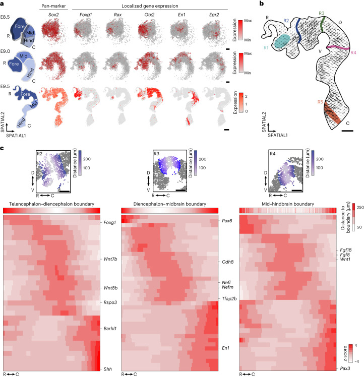
Spatiotemporal orchestration of gene expression is required for proper embryonic development. The use of single-cell technologies has begun to provide improved resolution of early regulatory dynamics, including detailed molecular definitions of most cell states during mouse embryogenesis. Here we used Slide-seq to build spatial transcriptomic maps of complete embryonic day (E) 8.5 and E9.0, and partial E9.5 embryos. To support their utility, we developed sc3D, a tool for reconstructing and exploring three-dimensional 'virtual embryos', which enables the quantitative investigation of regionalized gene expression patterns. Our measurements along the main embryonic axes of the developing neural tube revealed several previously unannotated genes with distinct spatial patterns. We also characterized the conflicting transcriptional identity of 'ectopic' neural tubes that emerge in Tbx6 mutant embryos. Taken together, we present an experimental and computational framework for the spatiotemporal investigation of whole embryonic structures and mutant phenotypes.

Fig. 1. Embryo-wide profiling of gene expression with spatial coordinates using Slide-seq.

a, Schematic of the experimental workflow and data analysis. Sagittal sections of mouse embryos at E8.5, E9.0 and E9.5 were obtained for Slide-seq. The dotted lines indicate the approximate position of the embryonic sections. b,c, 3D-reconstructed E8.5 (b) and E9.0 (c) stage embryos with six cell states highlighted (brain, heart, neural tube, somites, NMPs, PSM); the caudal marker gene Cdx2 and heart tube marker gene Ttn are shown (normalized gene expression) in a vISH of the reconstructed E8.5 embryo1. Each dot corresponds to a single bead. Point of view is denoted by the eye symbol. Scale bars, 100 µm. d, 3D view of an E8.5 embryo showing the indicated cell states and anatomical features in brightfield (left) or mapped onto the E8.5 embryo1 (right). Different orientations are displayed. Scale bars, 500 µm. e, Schematic of the strategy used to identify localized gene expression in tissues. f, Heatmap of localization scores for the top 20 spatially differentially expressed genes in 3D for each analyzed tissue in the E8.5 embryo1 (see Supplementary Table 4 for the list). Top 20 genes (row z-score-normalized) in the brain are highlighted. A, anterior; LPM, lateral plate mesoderm; P, posterior; D, dorsal; V, ventral; LPM, lateral plate mesoderm; NMPs, neuromesodermal progenitors; PSM, pre-somitic mesoderm.

Fig. 2. Localized gene expression patterns in the developing brain.

a, Schematic (left) and normalized gene expression spatial plot (right) of selected genes (highlighted in Fig. 1f) in the 3D brain of E8.5 embryo1, E9.0 and E9.5 (array E9.5_3). Each dot represents a single bead. b, Spatial plot of RNA velocity in the E9.5 (array E9.5_3) brain region. Vector direction indicates the trajectory and length denotes the magnitude. Low-velocity regions are indicated as R1, R2, R3 and R4. R1, neural ridge prosencephalon; R2, telencephalon–diencephalon boundary; R3, diencephalon–mesencephalon boundary; R4: mesencephalon–hindbrain boundary; and R5, hindbrain–spinal cord boundary. c, Spatial plot showing the brain boundaries (top) and top enriched spatially differentially expressed genes along the R2, R3 and R4 brain boundaries (represented as row z-score-normalized expression) at E9.5 (array E9.5_3). The full list of genes can be found in Supplementary Table 5. Scale bar for all plots, 50 µm. C, caudal; D, dorsal; R, rostral; V, ventral.

Fig. 3. Spatial organization of the embryonic trunk.

a, Schematic of the spatial organization of cell states in the embryonic trunk region at E8.5, and close-up view on the somitogenesis process. b, Schematic and 3D spatial plot of E8.5 (embryo2), showing selected cell states and vISH of Tbx6, Ripply2 and Meox1 in the trunk region. Each dot denotes a bead and the color corresponds to the indicated state. Scale bar, 200 µm. c, UMAP showing beads from E8.5 and E9.5 embryos corresponding to the NMPs, PSM, somites and neural tube states (left) and the corresponding spatial distribution (right) in an E9.5 embryo (array E9.5_2). Each dot denotes a bead and the color corresponds to the indicated state. Scale bar, 100 µm. d, UMAP showing pseudotime analysis along the somitic and neural differentiation trajectories (left) and the corresponding spatial distribution (right) in an E9.5 embryo (array E9.5_2). Each dot denotes a bead and the color corresponds to the assigned pseudotime value. Scale bar, 100 µm. e, Density plot displaying the computed pseudotime difference (y axis) versus the measured spatial distance (x axis) between all beads of the same cell state. Each dot is a pairwise comparison. The dotted line delineates cells with low spatial distance and large transcriptional divergence in the neural tube. f, Spatial plot showing the beads (top) within the dotted line (Fig. 2e) and the distribution of pseudotime values in an E9.5 embryonic trunk (array E9.5_3) that reflects neural tube patterning. Each dot represents a bead. Scale bars, 100 µm.

Fig. 4. Neural tube profiling along the AP and DV axes.

a, Schematic of an E9.5 stage embryo, with beads corresponding to the neural tube (green) and the denoted axes along which profiling was performed (array E9.5_10). b, Heatmap showing the top 160 genes with expression patterns (row z-score-normalized, filtered for a log fold change greater than 0.05 and a false discovery rate (FDR) < 0.01; see Supplementary Table 7 for the list of genes) in the 25 generated spatial bins along the AP axis. Expression of Hox genes is highlighted (right). Scale bar, 184 µm. c, Spatial plots showing the normalized expression (bin z-score) of Hox modules (I, II, III, IV, V, VI) in the E9.5 (array E9.5_10) neural tube. Two representative genes for each module are indicated. Scale bar, 100 µm. d, Heatmap showing the top 160 genes with expression patterns (row z-score-normalized, filtered for a log fold change greater than 0.05 and FDR < 0.01; see Supplementary Table 7 for the list of genes) in the eight generated spatial bins along the DV axis. Expression of known patterned and our identified genes are highlighted. Scale bar, 40 µm. e, RNA–FISH showing validation for known (top) and our identified (bottom) patterns along the DV axis of the neural tube. A single tissue slice obtained from the posterior portion of the neural tube is shown in the images. n = 3 embryos with reproducible staining pattern for each profiled target from WT embryos. Scale bars, 50 µm. f, Schematic showing the spatial patterns of known (within the tube) and our identified (outside the tube) genes along the DV axis of the E9.5 stage neural tube.

Fig. 5. Slide-seq profiling of Tbx6 KO embryos.

a, Transverse section of DAPI stained embryos (top) and spatial plot (bottom) showing the annotated tissue morphologies (somites, neural tube) and corresponding cell states in E9.5 WT and KO embryo. The KO experiment was independently performed five times in total with n > 5 embryos per experiment, and consistently yielded the same phenotype. The Slide-seq experiment was performed on one representative transversal section for WT and two for KO embryos. b, Spatial grid map showing the organization of neural tube 1, 2 and somitic cells in WT and Tbx6 KO embryos. c, UMAP showing the projection of cells assigned to the indicated clusters on the trunk trajectory (Fig. 3c), with the size of the dots representing the degree of uncertainty of mapping to the respective position. d, Dot plot showing the expression of the indicated genes in the three clusters (dot size is percentage of cells per cluster; color is cluster average normalized expression). e, RNA–FISH of the indicated genes in a transversal section of an E9.5 WT and KO embryos. The dotted lines in the schematic denote the AP position within the trunk from which sections were obtained. A representative section from WT and KO embryos at E9.5 is shown. The expression pattern was verified in two of the KO experiments with n > 3 embryos per experiment. Scale bars, 50 µm. f, Schematic showing the transcriptional identity and patterning characteristic of the ectopic neural tubes that arise in the absence of Tbx6 expression, highlighting their conflicting transcriptional identity.

Extended Data Fig. 1. Integration and cell-type annotation.

a. Brightfield images of representative embryos isolated from 3 independent foster mice and staged for the respective developmental stages. Scale bar, 500 µm. b. Distribution of beads profiled by Slide-seq from the respective stages. c. Violin plots showing the number of UMIs or genes recovered per bead. Log₁₀ values are used to represent counts. UMI, unique molecular identifier. d. Violin plots showing the number of UMIs and genes recovered per bead across individual arrays. Log₁₀ values are used to represent counts. UMI, unique molecular identifier. e. Uniform Manifold Approximation and Projection (UMAP) of Slide-seq data and 10X scRNA-seq reference atlas of mouse gastrulation. The color of the beads corresponds to the predicted and annotated cell state. Inset: UMAP representation of beads covered by the indicated modalities (red). Each dot represents a bead or a cell. f. UMAP of integrated data from stages E6.5 to E9.5. Black beads represent cells/beads from the corresponding stage. Each dot represents a bead or a cell.

Extended Data Fig. 2. Spatial organization of cell states.

a. Representative trunk/thoracic array (array E9.5_2) with highlighted cell states projected spatially. Each dot represents a bead. Outlines are used to emphasize morphological characteristics. A, anterior; P, posterior; D, dorsal; V, ventral. Scale bar, 200 μm b. Comparison of Slide-seq and conventional whole-mount in situ hybridization for gene expression patterns. Spatial gene expression plot showing the expression of Ttn (heart), Sox2 (neural tube), T (tailbud mesoderm), and Meox1 (somites). The color scale depicts normalized gene expression. n/n in the whole-mount in situ hybridization panel indicates the number of embryos exhibiting the pattern to the total number of embryos assayed (from one experiment). Each dot represents a bead. Scale bar, 200 μm. c. Cell states distribution of annotated clusters in the individual E9.5 arrays. Colors represent individual cell states, legend in panel (d). d. Spatial projection of annotated cell states in E9.5 embryo arrays. The panel depicts arrays that cover the trunk/thoracic and head regions. Each color corresponds to a distinct cell state. Each dot represents a bead. Scale bar, 200 μm. A, anterior; P, posterior; D, dorsal; V, ventral; R, rostral; C, caudal. e. Cell state distribution of the annotated clusters in individual arrays of the two independently profiled whole E8.5 stage embryos. Colors represent individual cell states according to the legend in panel (d). f. Cell state distribution of individual states in 10X scRNA-seq reference and Slide-seq at E8.5 stage (left panel), and the comparison between the two whole E8.5 embryos profiled by Slide-seq (right panel).

Extended Data Fig. 3. E8.5 and E9.0 3D embryos.

a, b. Spatial projection of cell states in individual arrays of the two whole E8.5 embryos. Each dot corresponds to a bead. Each color represents a cell state. Scale bar, 200 μm. c-d. Volumes of the indicated tissues ranked from the largest to the smallest, calculated from the E8.5 and E9.0 3D virtual embryo. Tissue volumes are listed in Supplementary Table 2. e. Relative volume of each tissue in the two whole E8.5 embryos. f. Disagreement between the initial and skipped slices when increasing the distance between individual slices.

Extended Data Fig. 4. Robustness of sc3D.

a, b. Comparison of accuracy and processing time (sc3D vs PASTE) across different datasets. c. Boxplot of the pairwise distances between the beads in the correctly registered images and those generated by the algorithm when slices are separated by 60, 90, 120, 150, 180, 210 µm (‘n’ slice pairs: 6,4,3,3,2,1, respectively). Boxplot elements: middle line, median; box plot limits, upper and lower quartiles; whiskers, standard deviation. d. Barplot of the overlap of localized genes across tissues in the two individual E8.5 whole embryos. Complete list of genes can be found in Supplementary Table 3. e. Barplot of the fraction of localized genes in the individual 2D arrays that were in the top 10 ranked localized genes in 3D volume of the respective tissues across all tissues in the E8.5 embryo (shown is the analysis for E8.5_Embryo_1). Error bars denote standard deviation of genes between the 2D slices and 3D volume (n = 13 genes). f-g. Heatmap of top localized genes (row z-score normalization) across the indicated tissues in the E8.5 embryo_1 (f) and E9.0 (g) embryo.

Extended Data Fig. 5. Localized gene expression in the developing heart.

a. 3D view of E8.5 embryo highlighting the heart tissue volume (in pink). Each dot corresponds to a bead. The point of view is denoted by the eye symbol (yellow or blue). b. Scatter plot showing the top localized genes in the heart tissue volume. Color scale corresponds to localization score ranging from 0.06 (light red) to 0.30 (dark red). Each dot represents a gene. Spatial localization of the highlighted genes is displayed in c. x-axis shows the density of gene expression, and y-axis shows the relative volume of expression within the tissue. c. vISH of localized genes, Nppa, Cck, Sfrp5 and Tdgf1. Color scale denotes the normalized gene expression values ranging from minimum to maximum for every gene. Each dot corresponds to a bead. The point of view is denoted by the eye symbol (yellow or blue). RNA-FISH in the E9.0 embryo shows the distinct localization of Tdgf1 in the heart. Scale bar, 100 µm. d. vISH showing gene co-expression for Cck (magenta) and Sfrp5 (green) in the heart tissue. Each dot corresponds to a bead. Color scale for each gene ranges from black to magenta, or black to green. Beads double-positive are displayed in white. e. vISH for spatially ubiquitous genes in the state ‘primitive blood late’. Scale bar, 200 µm. A, anterior; P, posterior; D, dorsal; V, ventral; L, left; R, right.

Extended Data Fig. 6. Spatial organization in the developing brain.

a. Spatial plot of the annotated clusters/states in the brain region of an E9.5 stage embryo (array E9.5_5). Each dot corresponds to a bead. Each color represents the annotated cell state. Scale bar, 200 µm. b. Spatial gene expression plot depicting the indicated genes of the mentioned categories. Each dot represents a bead. The color scale depicts normalized gene expression. Scale bar, 200 µm. Array shown is E9.5_3. c. Dotplot showing the expression of mid and hindbrain genes (annotated in the mid and hindbrain clusters in this study). Size of the dot represents the percentage of cells expressing the genes, and the color denotes the normalized gene expression. d. Volcano plot of the differentially expressed genes between the annotated mid and hindbrain (this study). Each dot represents a gene, dots in grey are below the significance threshold (genes filtered by FDR < 0.01 and logFC>0.2; Two-sided Wilcoxon ran sum test). e. Schematic and spatial expression plot distinguishing dorsal and ventral diencephalon/midbrain regions. Shh marks the ventral domain, whereas Fzd10 (Wnt receptor) marks the dorsal part. Each dot represents a bead. The color scale depicts normalized gene expression. Scale bar, 100 µm. D, dorsal; V, ventral; R, rostral; C, caudal.

Extended Data Fig. 7. Patterning of the developing brain.

a. Spatial velocity length (left) and confidence of directionality (right) highlight regions with different dynamics. Scale bar, 200 µm. Array shown is E9.5_3. b. Combining the length and confidence measurement results in ‘low’ and ‘high’ velocity regions. Regions with ‘low’ velocity display lower length and lower directionality. Regions with ‘high’ velocity display higher length and directionality of the vector. Scale bar is 200 µm. Array shown is E9.5_3. c. Inset regions of the RNA velocity in the brain region with expression of markers defining the respective boundary regions (representative of 3 independent E9.5 arrays). Each dot corresponds to a bead. Color scale denotes normalized expression. Scale bar, 50 µm. d. Spatial plot of WNT genes at R2 (Telencephalon-diencephalon boundary – denoted arrows; representative of 3 independent E9.5 arrays). Each dot corresponds to a bead. Color scale denotes normalized expression. Scale bar, 50 µm. e. Slide-seq based schematic of the developing eye. The forebrain (dark blue) and the eye (orange) are depicted with the fraction of beads corresponding to each state (bar plot). 1499/4824 beads for the forebrain/anterior neural tube; 105/4824 beads for the eye/anterior neural tube; and 105/1499 beads for the eye/forebrain. Spatial plot showing the expression of the eye-specific marker Six6. A, anterior; R, rostral; C, caudal; D, dorsal; V, ventral. f. Spatial plots showing the expression of two newly identified eye marker genes, Cp and Vwc2 (left: whole E9.5_3 array; middle: subset of the ‘eye’; right: RNA-FISH validations for Cp and Vwc2 (magenta) and counterstained nuclei (grey) are shown for a representative embryo. n = 3 embryos/experiment, 3 independent experiments). Scalebar, 200 µm. R, rostral; C, caudal; D, dorsal; V, ventral.

Extended Data Fig. 8. Transcriptional dynamics in the trunk region.

a. Spatial plot showing beads from E9.5 embryo (array E9.5_6) corresponding to the NMPs, PSM, somites and neural tube clusters (left panel) and the corresponding pseudotime values (right panel). Each dot corresponds to a bead. Cell states are highlighted in the indicated colors. Scale bar, 200 µm. b. Heatmap showing the expression of pseudotime determining genes along the somitic and neural trajectories. Genes used for the heatmap are listed in Supplementary Table 6. c. Line plot showing gene expression of selected genes along the neural and somitic trajectories. y-axis represents scaled gene expression. d. Schematic workflow of the ‘axis profiling’ tool. e. Pie chart displaying differentially expressed genes along the anteroposterior axis divided by cellular and molecular function. Genes are listed in Supplementary Table 7. f. Line plot showing the spatial distribution along the anterior-posterior axis of the Hox modules’ expression (I-VI). g. vISH for Hox genes in 3D virtual E9.0 stage embryo. Scale bar, 200 µm. D, dorsal; V, ventral; A, anterior; P, posterior.

Extended Data Fig. 9. Neural tube dorsoventral patterning.

a. Heatmap showing the top 160 genes with gene expression regionalization in one of the eight generated bins along the dorsoventral axis (genes filtered by FDR < 0.01 and logFC>0.05 then ranked by FDR). A selected set of previously known genes associated with dorsoventral patterning (black) are highlighted on the right. Specific structures along the axis are highlighted at the bottom of the heatmap. Genes are row z-score normalized and listed in Supplementary Table 7. b. Heatmap showing column scaled z-score of Pearson correlation coefficients comparing the Slide-seq dorsoventral bins and the identified clusters from a neural tube single-cell reference. RP, roof plate; dp, dorsal progenitors; pMN, motor neuron progenitors; FP, floor plate. c. Heatmap showing an extended subset of the genes that display gene expression regionalization in one of the eight generated bins along the dorsoventral axis (genes filtered by FDR < 0.01 and logFC>0.05 then ranked by FDR). Specific structures along the axis are highlighted at the bottom of the heatmap. Genes are row z-score normalized and listed in Supplementary Table 7. d. Pie chart displaying differentially expressed genes along the dorsoventral axis divided by cellular and molecular function. Genes are listed in Supplementary Table 7. e. Schematic (top panel) and spatial gene expression plots of the known neural tube patterning genes in array E9.5_2. Each dot denotes a bead. The color scale depicts normalized gene expression. D, dorsal; V, ventral; A, anterior; P, posterior. f. RNA-FISH and Slide-seq quantifications for each profiled gene from Fig. 4e. Genes are bin z-score normalized (magenta: RNA-FISH; orange: Slide-seq). D, dorsal; V, ventral.

Extended Data Fig. 10. Tbx6-KO spatial profiling.

a. Schematic of Tbx6 gene ablation strategy. Guide RNAs target the denoted exons. UTR, untranslated region. b. Schematic showing the plane of cryosectioning for Slide-seq experiment. c. Spatial plot of all cell states in the complete WT and Tbx6-KO trunk transversal arrays. Dotted lines denote the region that was used for further analysis. Each dot corresponds to a bead. Each color represents an individual state. Scale bar, 200 µm. d. UMAP, spatial and fraction plot showing the filtered and de novo annotated cell states. e. Dot plot depicting the expression of neural tube and somitic marker genes in the somites, neural tube 1 and 2 clusters. The size of the dots represents the % of cells expressing the gene, and the color represents the cluster average normalized expression level. f. Scatter plot showing differentially expressed genes between somitic vs central tubes clusters and central vs ectopic tubes clusters (genes filtered by FDR < 0.01. Complete list of genes in Supplementary Table 9. g. RNA-FISH of Foxa2 and Pax6 in a transversal section of the neural tube in WT and Tbx6-KO embryos. The schematic represents the anteroposterior position where the transversal sections were profiled. Scale bar, 50 µm. D, dorsal; V, ventral; WT, wild type; KO, knockout.

References

1. Arnold SJ, Robertson EJ. Making a commitment: cell lineage allocation and axis patterning in the early mouse embryo. Nat. Rev. Mol. Cell Biol. 2009;10:91–103. doi: 10.1038/nrm2618. - DOI - PubMed
1. Rivera-Pérez, J. A. & Hadjantonakis, A.-K. The dynamics of morphogenesis in the early mouse embryo. Cold Spring Harb. Perspect. Biol.7, a015867 (2014). - PMC - PubMed
1. Selleck MA, Stern CD. Fate mapping and cell lineage analysis of Hensen’s node in the chick embryo. Development. 1991;112:615–626. doi: 10.1242/dev.112.2.615. - DOI - PubMed
1. Tam PP, Behringer RR. Mouse gastrulation: the formation of a mammalian body plan. Mech. Dev. 1997;68:3–25. doi: 10.1016/S0925-4773(97)00123-8. - DOI - PubMed
1. Tam PPL, Loebel DAF. Gene function in mouse embryogenesis: get set for gastrulation. Nat. Rev. Genet. 2007;8:368–381. doi: 10.1038/nrg2084. - DOI - PubMed
Publication types