Influence of electric field, blood velocity, and pharmacokinetics on electrochemotherapy efficiency

Abstract

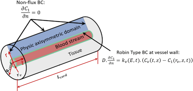
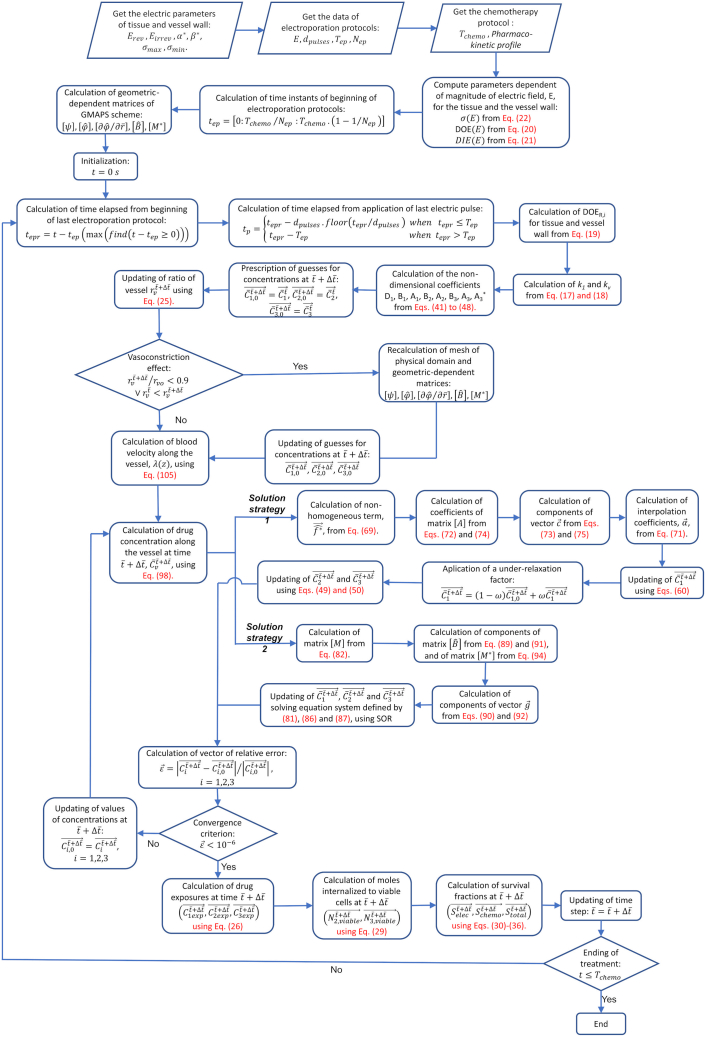
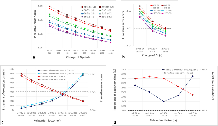
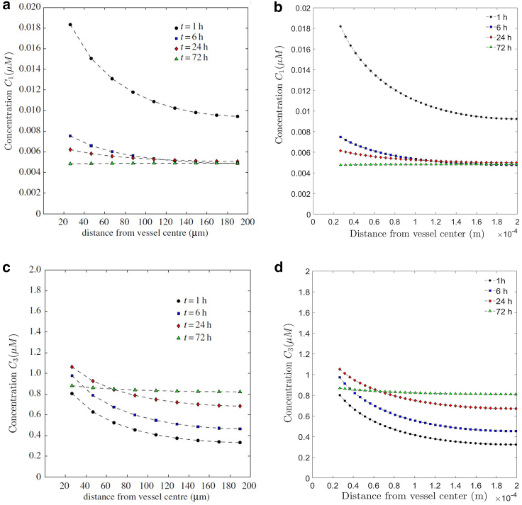
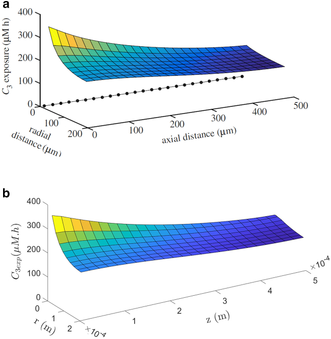
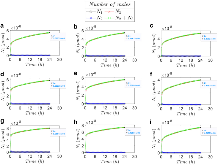
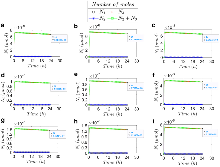
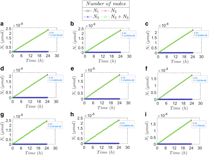
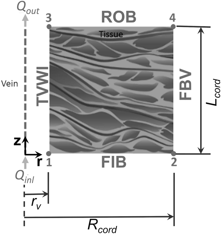
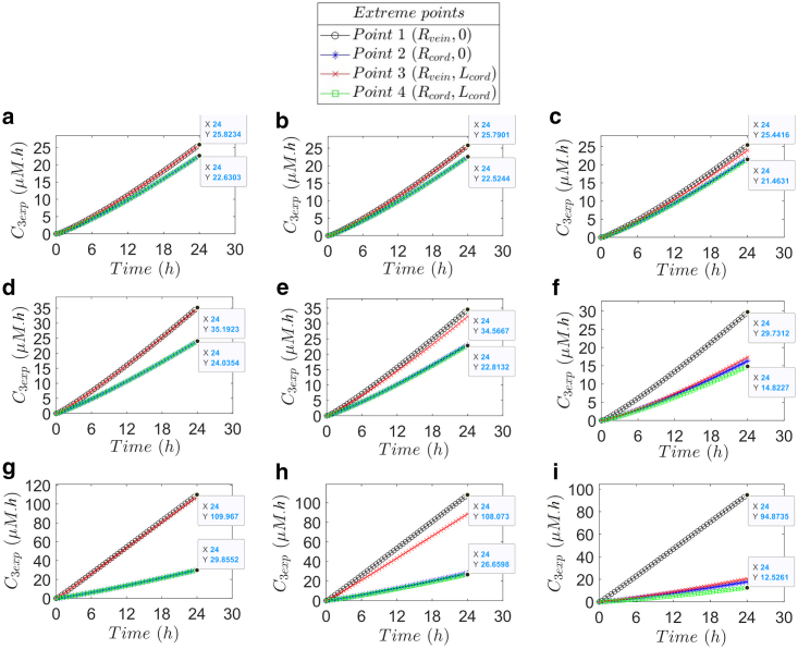
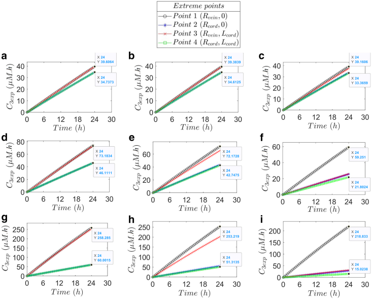
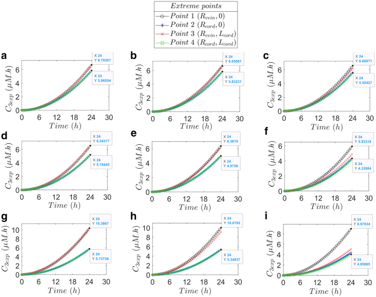
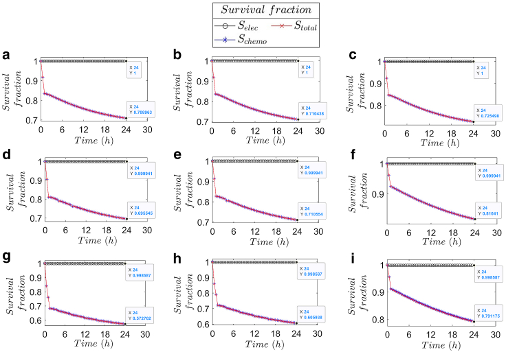
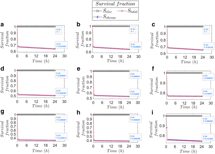
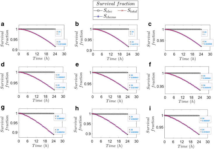
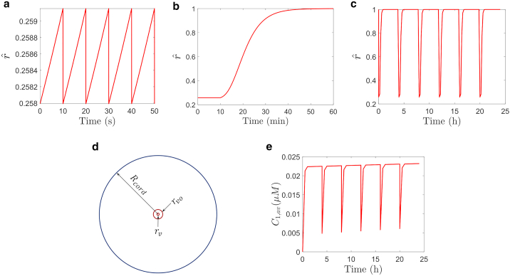
The convective delivery of chemotherapeutic drugs in cancerous tissues is directly proportional to the blood perfusion rate, which in turns can be transiently reduced by the application of high-voltage and short-duration electric pulses due to vessel vasoconstriction. However, electric pulses can also increase vessel wall and cell membrane permeabilities, boosting the extravasation and cell internalization of drug. These opposite effects, as well as possible adverse impacts on the viability of tissues and endothelial cells, suggest the importance of conducting in silico studies about the influence of physical parameters involved in electric-mediated drug transport. In the present work, the global method of approximate particular solutions for axisymmetric domains, together with two solution schemes (Gauss-Seidel iterative and linearization+successive over-relaxation), is applied for the simulation of drug transport in electroporated cancer tissues, using a continuum tumor cord approach and considering both the electropermeabilization and vasoconstriction phenomena. The developed global method of approximate particular solutions algorithm is validated with numerical and experimental results previously published, obtaining a satisfactory accuracy and convergence. Then, a parametric study about the influence of electric field magnitude and inlet blood velocity on the internalization efficacy, drug distribution uniformity, and cell-kill capacity of the treatment, as expressed by the number of internalized moles into viable cells, homogeneity of exposure to bound intracellular drug, and cell survival fraction, respectively, is analyzed for three pharmacokinetic profiles, namely one-short tri-exponential, mono-exponential, and uniform. According to numerical results, the trade-off between vasoconstriction and electropermeabilization effects and, consequently, the influence of electric field magnitude and inlet blood velocity on the assessment parameters considered here (efficacy, uniformity, and cell-kill capacity) is different for each pharmacokinetic profile deemed.

Figure 1

For a Figure360 author presentation of Fig. 1, see https://doi.org/10.1016/j.bpj.2023.07.004. Boundary conditions of the physical domain. To see this figure in color, go online.

Figure 2

General behavior of transient degree of electroporation (${DOE}_{R,i}$) with the normalized electric field (${\raisebox{1ex}{$E$}\!\left/ \!\raisebox{-1ex}{$E$}\right.}_{irrev}$). To see this figure in color, go online.

Figure 3

(a) Plot of $r_v/r_{v0}$ vs. $t_p/{\tau }_r$ for several values of $m_r.E$ obtained with the present model. (b) Plots of normalized diameter versus time for several pulse frequencies experimentally obtained by (23). (c) Plot of $r_v/r_{v0}$ vs. $m_r.E$ for $t_p=0\mathrm{s}$ obtained with the present model, where the asymptotic behavior can be appreciated. (d) Plots of normalized diameter versus pulse amplitude experimentally obtained by (23), where the asymptotic behavior can be confirmed. To see this figure in color, go online.

Figure 5

Graphical scheme of the field smoothing. To see this figure in color, go online.

Figure 4

Basic flowchart of iterative GMAPS solution scheme. To see this figure in color, go online.

Figure 6

(a) Plot of $L^2$ versus change of $N_{points}$ for several values of $\Delta t$. (b) Plot of $L^2$ versus change of $\Delta t$ for several values of $N_{points}$. (c) Plot of convergence on the relaxation factor ($\omega$) and increment in execution time for S1. (d) Plot of convergence on the relaxation factor ($\omega$) and increment in execution time for S2. To see this figure in color, go online.

Figure 7

Comparison between $FVM$ (42) and $GMAPS$ solution. (a) Extracellular concentrations $\left(C_1\right)$ obtained by $FVM$. (b) Extracellular concentrations $\left(C_1\right)$ obtained by $GMAPS$. (c) Intracellular bound concentrations $\left(C_3\right)$ obtained by $FVM$. (d) Intracellular bound concentrations $\left(C_3\right)$ obtained by $GMAPS$. To see this figure in color, go online.

Figure 8

Exposure to bound intracellular drug: comparison of results (a) $FVM$ (28) and (b) $GMAPS$. To see this figure in color, go online.

Figure 9

Number of moles versus time. (a) $E=0\mathrm{k}\mathrm{V}/\mathrm{m}$, $\lambda =1\times {10}^{-2}\mathrm{m}/\mathrm{s}$, PK = one short tri-exponential. (b) $E=0\mathrm{k}\mathrm{V}/\mathrm{m}$, $\lambda =1\times {10}^{-3}\mathrm{m}/\mathrm{s}$, PK = one short tri-exponential. (c) $E=0\mathrm{k}\mathrm{V}/\mathrm{m}$, $\lambda =1\times {10}^{-4}\mathrm{m}/\mathrm{s}$, PK = one short tri-exponential. (d) $E=46\mathrm{k}\mathrm{V}/\mathrm{m}$, $\lambda =1\times {10}^{-2}\mathrm{m}/\mathrm{s}$, PK = one short tri-exponential. (e) $E=46\mathrm{k}\mathrm{V}/\mathrm{m}$, $\lambda =1\times {10}^{-3}\mathrm{m}/\mathrm{s}$, PK = one short tri-exponential. (f) $E=46\mathrm{k}\mathrm{V}/\mathrm{m}$, $\lambda =1\times {10}^{-4}\mathrm{m}/\mathrm{s}$, PK = one short tri-exponential. (g) $E=70\mathrm{k}\mathrm{V}/\mathrm{m}$, $\lambda =1\times {10}^{-2}\mathrm{m}/\mathrm{s}$, PK = one short tri-exponential. (h) $E=70\mathrm{k}\mathrm{V}/\mathrm{m}$, $\lambda =1\times {10}^{-3}\mathrm{m}/\mathrm{s}$, PK = one short tri-exponential. (i) $E=70\mathrm{k}\mathrm{V}/\mathrm{m}$, $\lambda =1\times {10}^{-4}\mathrm{m}/\mathrm{s}$, PK = one short tri-exponential. To see this figure in color, go online.

Figure 10

Number of moles versus time. (a) $E=0\mathrm{k}\mathrm{V}/\mathrm{m}$, $\lambda =1\times {10}^{-2}\mathrm{m}/\mathrm{s}$, PK = mono-exponential. (b) $E=0\mathrm{k}\mathrm{V}/\mathrm{m}$, $\lambda =1\times {10}^{-3}\mathrm{m}/\mathrm{s}$, PK = mono-exponential. (c) $E=0\mathrm{k}\mathrm{V}/\mathrm{m}$, $\lambda =1\times {10}^{-4}\mathrm{m}/\mathrm{s}$, PK = mono-exponential. (d) $E=46\mathrm{k}\mathrm{V}/\mathrm{m}$, $\lambda =1\times {10}^{-2}\mathrm{m}/\mathrm{s}$, PK = mono-exponential. (e) $E=46\mathrm{k}\mathrm{V}/\mathrm{m}$, $\lambda =1\times {10}^{-3}\mathrm{m}/\mathrm{s}$, PK = mono-exponential. (f) $E=46\mathrm{k}\mathrm{V}/\mathrm{m}$, $\lambda =1\times {10}^{-4}\mathrm{m}/\mathrm{s}$, PK = mono-exponential. (g) $E=70\mathrm{k}\mathrm{V}/\mathrm{m}$, $\lambda =1\times {10}^{-2}\mathrm{m}/\mathrm{s}$, PK = mono-exponential. (h) $E=70\mathrm{k}\mathrm{V}/\mathrm{m}$, $\lambda =1\times {10}^{-3}\mathrm{m}/\mathrm{s}$, PK = mono-exponential. (i) $E=70\mathrm{k}\mathrm{V}/\mathrm{m}$, $\lambda =1\times {10}^{-4}\mathrm{m}/\mathrm{s}$, PK = mono-exponential. To see this figure in color, go online.

Figure 11

Number of moles versus time. (a) $E=0\mathrm{k}\mathrm{V}/\mathrm{m}$, $\lambda =1\times {10}^{-2}\mathrm{m}/\mathrm{s}$, PK = uniform. (b) $E=0\mathrm{k}\mathrm{V}/m$, $\lambda =1\times {10}^{-3}\mathrm{m}/\mathrm{s}$, PK = uniform. (c) $E=0\mathrm{k}\mathrm{V}/\mathrm{m}$, $\lambda =1\times {10}^{-4}\mathrm{m}/\mathrm{s}$, PK = uniform. (d) $E=46\mathrm{k}\mathrm{V}/\mathrm{m}$, $\lambda =1\times {10}^{-2}\mathrm{m}/\mathrm{s}$, PK = uniform. (e) $E=46\mathrm{k}\mathrm{V}/\mathrm{m}$, $\lambda =1\times {10}^{-3}\mathrm{m}/\mathrm{s}$, PK = uniform. (f) $E=46\mathrm{k}\mathrm{V}/\mathrm{m}$, $\lambda =1\times {10}^{-4}\mathrm{m}/\mathrm{s}$, PK = uniform. (g) $E=70\mathrm{k}\mathrm{V}/\mathrm{m}$, $\lambda =1\times {10}^{-2}\mathrm{m}/\mathrm{s}$, PK = uniform. (h) $E=70\mathrm{k}\mathrm{V}/m$, $\lambda =1\times {10}^{-3}\mathrm{m}/\mathrm{s}$, PK = uniform. (i) $E=70\mathrm{k}\mathrm{V}/\mathrm{m}$, $\lambda =1\times {10}^{-4}\mathrm{m}/\mathrm{s}$, PK = uniform. To see this figure in color, go online.

Figure 12

Extreme points of the tumor cord domain.

Figure 13

Exposure to bound intracellular drug $\left(C_{3\mathit{exp}}\right)$ versus time. (a) E = 0 kV/m, $\lambda =1\times {10}^{-2}\mathrm{m}/\mathrm{s}$, PK = one short tri-exponential. (b) E = 0 kV/m, $\lambda =1\times {10}^{-3}\mathrm{m}/\mathrm{s}$, PK = one short tri-exponential. (c) E = 0 kV/m, $\lambda =1\times {10}^{-4}\mathrm{m}/\mathrm{s}$, PK = one short tri-exponential. (d) E = 46 kV/m, $\lambda =1\times {10}^{-2}\mathrm{m}/\mathrm{s}$, PK = one short tri-exponential. (e) E = 46 kV/m, $\lambda =1\times {10}^{-3}\mathrm{m}/\mathrm{s}$, PK = one short tri-exponential. (f) E = 46 kV/m, $\lambda =1\times {10}^{-4}\mathrm{m}/\mathrm{s}$, PK = one short tri-exponential. (g) E = 70 kV/m, $\lambda =1\times {10}^{-2}\mathrm{m}/\mathrm{s}$, PK = one short tri-exponential. (h) E = 70 kV/m, $\lambda =1\times {10}^{-3}\mathrm{m}/\mathrm{s}$, PK = one short tri-exponential. (i) E = 70 kV/m, $\lambda =1\times {10}^{-4}\mathrm{m}/\mathrm{s}$, PK = one short tri-exponential.

Figure 14

Exposure to bound intracellular drug $\left(C_{3\mathit{exp}}\right)$ versus time. (a) E = 0 kV/m, $\lambda =1\times {10}^{-2}\mathrm{m}/\mathrm{s}$, PK = mono-exponential. (b) E = 0 kV/m, $\lambda =1\times {10}^{-3}\mathrm{m}/\mathrm{s}$, PK = mono-exponential. (c) E = 0 kV/m, $\lambda =1\times {10}^{-4}\mathrm{m}/\mathrm{s}$, PK = mono-exponential. (d) E = 46 kV/m, $\lambda =1\times {10}^{-2}\mathrm{m}/\mathrm{s}$, PK = mono-exponential. (e) E = 46 kV/m, $\lambda =1\times {10}^{-3}\mathrm{m}/\mathrm{s}$, PK = mono-exponential. (f) E = 46 kV/m, $\lambda =1\times {10}^{-4}\mathrm{m}/\mathrm{s}$, PK = mono-exponential. (g) E = 70 kV/m, $\lambda =1\times {10}^{-2}\mathrm{m}/\mathrm{s}$, PK = mono-exponential. (h) E = 70 kV/m, $\lambda =1\times {10}^{-3}\mathrm{m}/\mathrm{s}$, PK = mono-exponential. (i) E = 70 kV/m, $\lambda =1\times {10}^{-4}\mathrm{m}/\mathrm{s}$, PK = mono-exponential.

Figure 15

Exposure to bound intracellular drug $\left(C_{3\mathit{exp}}\right)$ versus time. (a) E = 0 kV/m, $\lambda =1\times {10}^{-2}\mathrm{m}/\mathrm{s}$, PK = uniform. (b) E = 0 kV/m, $\lambda =1\times {10}^{-3}\mathrm{m}/\mathrm{s}$, PK = uniform. (c) E = 0 kV/m, $\lambda =1\times {10}^{-4}\mathrm{m}/\mathrm{s}$, PK = uniform. (d) E = 46 kV/m, $\lambda =1\times {10}^{-2}\mathrm{m}/\mathrm{s}$, PK = uniform. (e) E = 46 kV/m, $\lambda =1\times {10}^{-3}\mathrm{m}/\mathrm{s}$, PK = uniform. (f) E = 46 kV/m, $\lambda =1\times {10}^{-4}\mathrm{m}/\mathrm{s}$, PK = uniform. (g) E = 70 kV/m, $\lambda =1\times {10}^{-2}\mathrm{m}/\mathrm{s}$, PK = uniform. (h) E = 70 kV/m, $\lambda =1\times {10}^{-3}\mathrm{m}/\mathrm{s}$, PK = uniform. (i) E = 70 kV/m, $\lambda =1\times {10}^{-4}\mathrm{m}/\mathrm{s}$, PK = uniform. To see this figure in color, go online.

Figure 16

Survival fraction versus time. (a) E = 0 kV/m, $\lambda =1\times {10}^{-2}\mathrm{m}/\mathrm{s}$, PK = One short tri-exponential. (b) E = 0 kV/m, $\lambda =1\times {10}^{-3}\mathrm{m}/\mathrm{s}$, PK = one short tri-exponential. (c) E = 0 kV/m, $\lambda =1\times {10}^{-4}\mathrm{m}/\mathrm{s}$, PK = one short tri-exponential. (d) E = 46 kV/m, $\lambda =1\times {10}^{-2}\mathrm{m}/\mathrm{s}$, PK = one short tri-exponential. (e) E = 46 kV/m, $\lambda =1\times {10}^{-3}\mathrm{m}/\mathrm{s}$, PK = one short tri-exponential. (f) E = 46 kV/m, $\lambda =1\times {10}^{-4}\mathrm{m}/\mathrm{s}$, PK = one short tri-exponential. (g) E = 70 kV/m, $\lambda =1\times {10}^{-2}\mathrm{m}/\mathrm{s}$, PK = one short tri-exponential. (h) E = 70 kV/m, $\lambda =1\times {10}^{-3}\mathrm{m}/\mathrm{s}$, PK = one short tri-exponential. (i) E = 70 kV/m, $\lambda =1\times {10}^{-4}\mathrm{m}/\mathrm{s}$, PK = one short tri-exponential. To see this figure in color, go online.

Figure 17

Survival fraction versus time. (a) E = 0 kV/m, $\lambda =1\times {10}^{-2}\mathrm{m}/\mathrm{s}$, PK = mono-exponential. (b) E = 0 kV/m, $\lambda =1\times {10}^{-3}\mathrm{m}/\mathrm{s}$, PK = mono-exponential. (c) E = 0 kV/m, $\lambda =1\times {10}^{-4}m/\mathrm{s}$, PK = mono-exponential. (d) E = 46 kV/m, $\lambda =1x{10}^{-2}\mathrm{m}/\mathrm{s}$, PK = mono-exponential. (e) E = 46 kV/m, $\lambda =1\times {10}^{-3}\mathrm{m}/\mathrm{s}$, PK = mono-exponential. (f) E = 46 kV/m, $\lambda =1\times {10}^{-4}\mathrm{m}/\mathrm{s}$, PK = mono-exponential. (g) E = 70 kV/m, $\lambda =1\times {10}^{-2}\mathrm{m}/\mathrm{s}$, PK = mono-exponential. (h) E = 70 kV/m, $\lambda =1\times {10}^{-3}\mathrm{m}/\mathrm{s}$, PK = mono-exponential. (i) E = 70 kV/m, $\lambda =1\times {10}^{-4}\mathrm{m}/\mathrm{s}$, PK = mono-exponential. To see this figure in color, go online.

Figure 18

Survival fraction versus time. (a) E = 0 kV/m, $\lambda =1\times {10}^{-2}\mathrm{m}/\mathrm{s}$, PK = uniform. (b) E = 0 kV/m, $\lambda =1\times {10}^{-3}\mathrm{m}/\mathrm{s}$, PK = uniform. (c) E = 0 kV/m, $\lambda =1\times {10}^{-4}\mathrm{m}/\mathrm{s}$, PK = uniform. (d) E = 46 kV/m, $\lambda =1\times {10}^{-2}\mathrm{m}/\mathrm{s}$, PK = uniform. (e) E = 46 kV/m, $\lambda =1\times {10}^{-3}\mathrm{m}/\mathrm{s}$, PK = uniform. (f) E = 46 kV/m, $\lambda =1\times {10}^{-4}\mathrm{m}/\mathrm{s}$, PK = uniform. (g) E = 70 kV/m, $\lambda =1\times {10}^{-2}\mathrm{m}/\mathrm{s}$, PK = uniform. (h) E = 70 kV/m, $\lambda =1\times {10}^{-3}\mathrm{m}/\mathrm{s}$, PK = uniform. (i) E = 70 kV/m, $\lambda =1\times {10}^{-4}\mathrm{m}/\mathrm{s}$, PK = uniform. To see this figure in color, go online.

Figure 19

(a) Plot of $\hat{r}$ versus t at timescale of pulse spacing. (b) Plot of $\hat{r}$ versus t at timescale of vessel radius recovery. (c) Plot of $\hat{r}$ versus t at timescale of electrochemotherapeutic treatment. (d) Graphical representation of vessel vasoconstriction. (e) Time evolution of the volume-averaged extracellular concentration $\left(C_{1,av}\right)$ for the uniform $PK$ profile and ${\lambda }_{inlet}=1\times {10}^{-4}\mathrm{m}/\mathrm{s}$.

References

1. Zhan W. 2014. Mathematical Modelling of Drug Delivery to Solid Tumour.
1. Fuso Nerini I., Morosi L., et al. D’Incalci M. Intratumor heterogeneity and its impact on drug distribution and sensitivity. Clin. Pharmacol. Ther. 2014;96:224–238. - PubMed
1. Tannock I.F., Lee C.M., et al. Egorin M.J. Limited penetration of anticancer drugs through tumor tissue: a potential cause of resistance of solid tumors to chemotherapy. Clin. Cancer Res. 2002;8:878–884. - PubMed
1. Batista Napotnik T., Miklavčič D. In vitro electroporation detection methods – An overview. Bioelectrochemistry. 2018;120:166–182. https://www.sciencedirect.com/science/article/pii/S156753941730395X?via%... - PubMed
1. Kotnik T., Rems L., et al. Miklavčič D. Membrane Electroporation and Electropermeabilization: Mechanisms and Models. Annu. Rev. Biophys. 2019;48:63–91. - PubMed
Publication types
LinkOut - more resources