Predictive power of non-identifiable models

Abstract

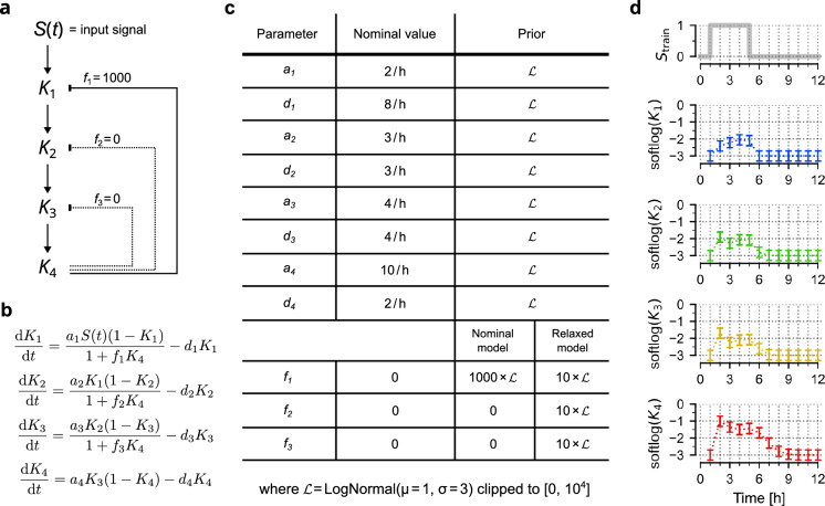
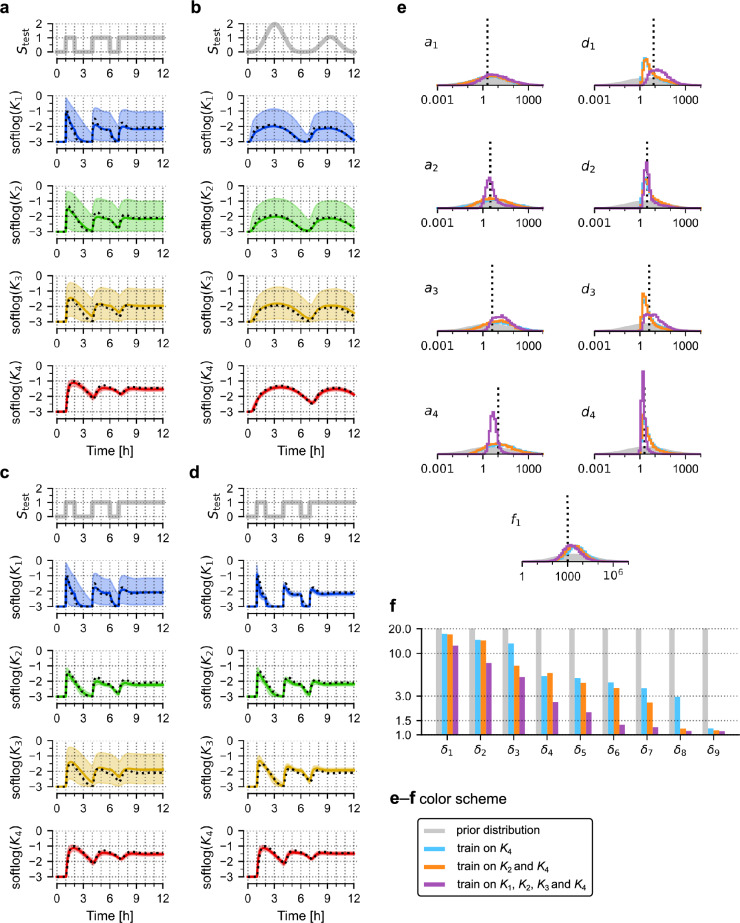
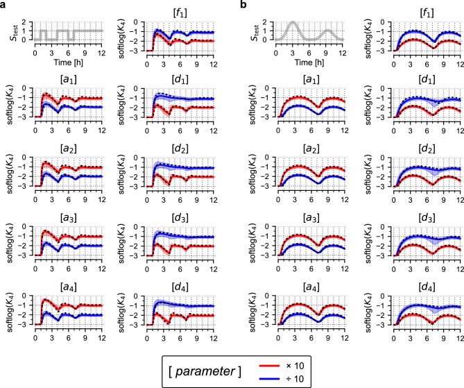
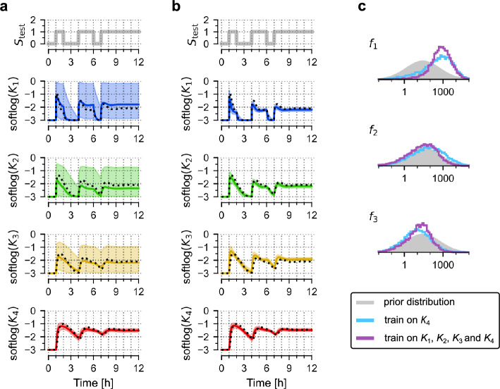
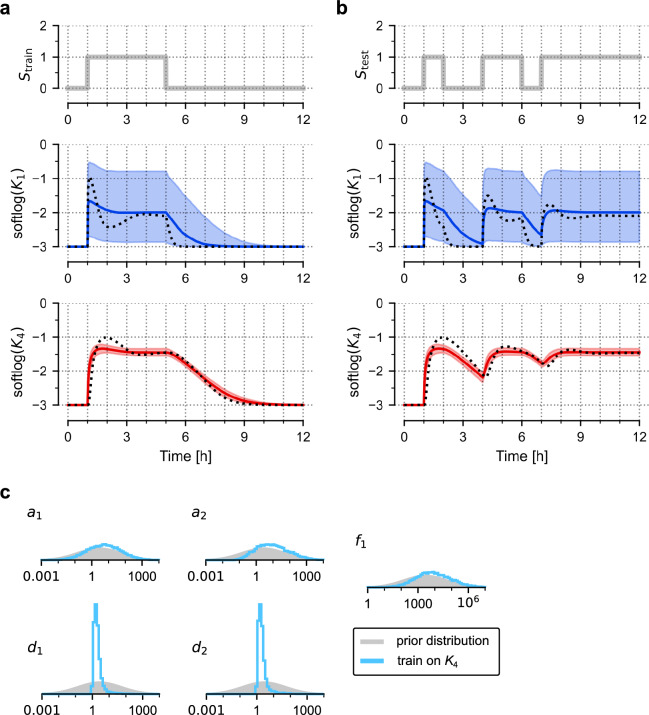
Resolving practical non-identifiability of computational models typically requires either additional data or non-algorithmic model reduction, which frequently results in models containing parameters lacking direct interpretation. Here, instead of reducing models, we explore an alternative, Bayesian approach, and quantify the predictive power of non-identifiable models. We considered an example biochemical signalling cascade model as well as its mechanical analogue. For these models, we demonstrated that by measuring a single variable in response to a properly chosen stimulation protocol, the dimensionality of the parameter space is reduced, which allows for predicting the measured variable's trajectory in response to different stimulation protocols even if all model parameters remain unidentified. Moreover, one can predict how such a trajectory will transform in the case of a multiplicative change of an arbitrary model parameter. Successive measurements of remaining variables further reduce the dimensionality of the parameter space and enable new predictions. We analysed potential pitfalls of the proposed approach that can arise when the investigated model is oversimplified, incorrect, or when the training protocol is inadequate. The main advantage of the suggested iterative approach is that the predictive power of the model can be assessed and practically utilised at each step.

Figure 1

Signalling cascade model. (a) Scheme of the 4-level biochemical signalling cascade model activated by a time-dependent signal S(t). Strengths of feedbacks f₂ and f₃ are set to zero in the nominal model but are allowed to assume positive values in the ‘relaxed’ model. (b) Model equations. (c) Model parameters used for generating training data and prior distributions used for training. (d) Simulated trajectories of K₁, K₂, K₃, and K₄ in response to S_train used for model training; softlog(x) = log(0.001 + x). Error bars show measurement errors assumed for the generation of training data.

Figure 2

Training the nominal model. (a,b) Prediction of model responses to two test signals, S_test, after training on the trajectory of K₄ (generated in response to the training protocol, S_train, shown in Fig. 1d). Black dotted lines show trajectories of the nominal model, coloured lines show (point-wise) medians of predictions, contours show 80% prediction bands; softlog(x) = log(0.001 + x). (c) Prediction of model responses after training on trajectories K₂ and K₄. (d) Prediction of model responses after training on trajectories of all four model variables, K₁, K₂, K₃ and K₄. (e) Histograms obtained from 10,000 samples generated from the posterior distribution of model parameters after training on K₄ (blue); K₂ and K₄ (orange); K₁, K₂, K₃ and K₄ (purple). Grey contours show prior distributions. (f) Dimensionality reduction of the parameter space by successive inclusion of model variable trajectories into the training set. Bar heights show principal multiplicative deviations δ_i = exp(√λ_i), where λ_i are principal values (variances) of log-parameters.

Figure 3

Predicted responses after changing model parameters. (a,b) Prediction of model responses to two test signals, S_test (shown in each panel top left), after training on the trajectory of K₄ (generated in response to the training protocol, S_train, shown in Fig. 1d). In each chart, one of the parameters (shown in square brackets) was multiplied (red) or divided (blue) by a factor of 10. Black dotted lines show trajectories of the nominal model, coloured lines show (point-wise) medians of predictions, contours show 80% prediction bands; softlog(x) = log(0.001 + x).

Figure 4

Training a relaxed model. (a) Prediction of model responses to test signal, S_test, after training on the trajectory of K₄ (generated in response to the training protocol, S_train, shown in Fig. 1d). Black dotted lines show trajectories of the nominal model, coloured lines show (point-wise) medians of predictions, contours show 80% prediction bands; softlog(x) = log(0.001 + x). (b) Prediction of model responses after training on trajectories of all four model variables. (c) Histograms were obtained from 10,000 samples generated from the posterior distribution of model parameters after training on K₄ (blue) or all model variables (purple). Grey contours show prior distributions.

Figure 5

Training a simplified model. (a) Training a simplified (2-step) model on the nominal (4-step) model trajectory of K₄. Only variables present in the simplified model are shown. Black dotted lines show trajectories of the nominal model, coloured lines show (point-wise) medians of the simplified model, contours show 80% prediction bands; softlog(x) = log(0.001 + x). (b) Prediction of the trained simplified model responses to the test signal, S_test. Same graphical convention as in (a). (c) Histograms were obtained from 10,000 samples generated from the posterior distribution of simplified model parameters. Grey contours show prior distributions.

Figure 6

Three-body harmonic oscillator. (a) Scheme of the model. All eight parameters (masses, m_i; damping coefficients b_i; spring constants k_i) to be estimated are given together with their nominal values. Before the time-dependent force F(t) is applied, the system remains in equilibrium. (b) Model equations. (c,d) Training (c) and prediction (d), with only the trajectory of the red mass included in the training. As in the signalling cascade model, for training, we use three independently generated measurement replicates with Gaussian noise (sigma σ_error = 0.3) added to the deterministic trajectory (black dotted line). Measurement points are at full seconds. Coloured lines show (point-wise) medians of predictions, contours show 80% prediction bands. (e,f) Training (e) and prediction (f), with trajectories of all masses included in the training, same convention as in (c,d). (g) Histograms were obtained from 10,000 samples generated from the posterior distribution of model parameters after training on red mass trajectory (red line) and after training on all masses trajectories (black line). Grey contours show (uniform) prior distributions.

References

1. Brown KS, Sethna JP. Statistical mechanical approaches to models with many poorly known parameters. Phys. Rev. E. 2003;68:021904. doi: 10.1103/PhysRevE.68.021904. - DOI - PubMed
1. Gutenkunst RN, et al. Universally sloppy parameter sensitivities in systems biology models. PLoS Comput. Biol. 2007;3:e189. doi: 10.1371/journal.pcbi.0030189. - DOI - PMC - PubMed
1. Raue A, et al. Structural and practical identifiability analysis of partially observed dynamical models by exploiting the profile likelihood. Bioinformatics. 2009;25:1923–1929. doi: 10.1093/bioinformatics/btp358. - DOI - PubMed
1. Wieland F-G, Hauber AL, Rosenblatt M, Tönsing C, Timmer J. On structural and practical identifiability. Curr. Opin. Syst. Biol. 2021;25:60–69. doi: 10.1016/j.coisb.2021.03.005. - DOI
1. Jaruszewicz-Błońska J, Kosiuk I, Prus W, Lipniacki T. A plausible identifiable model of the canonical NF-κB signaling pathway. PLoS ONE. 2023;18:e0286416. doi: 10.1371/journal.pone.0286416. - DOI - PMC - PubMed