A universal description of stochastic oscillators

Abstract

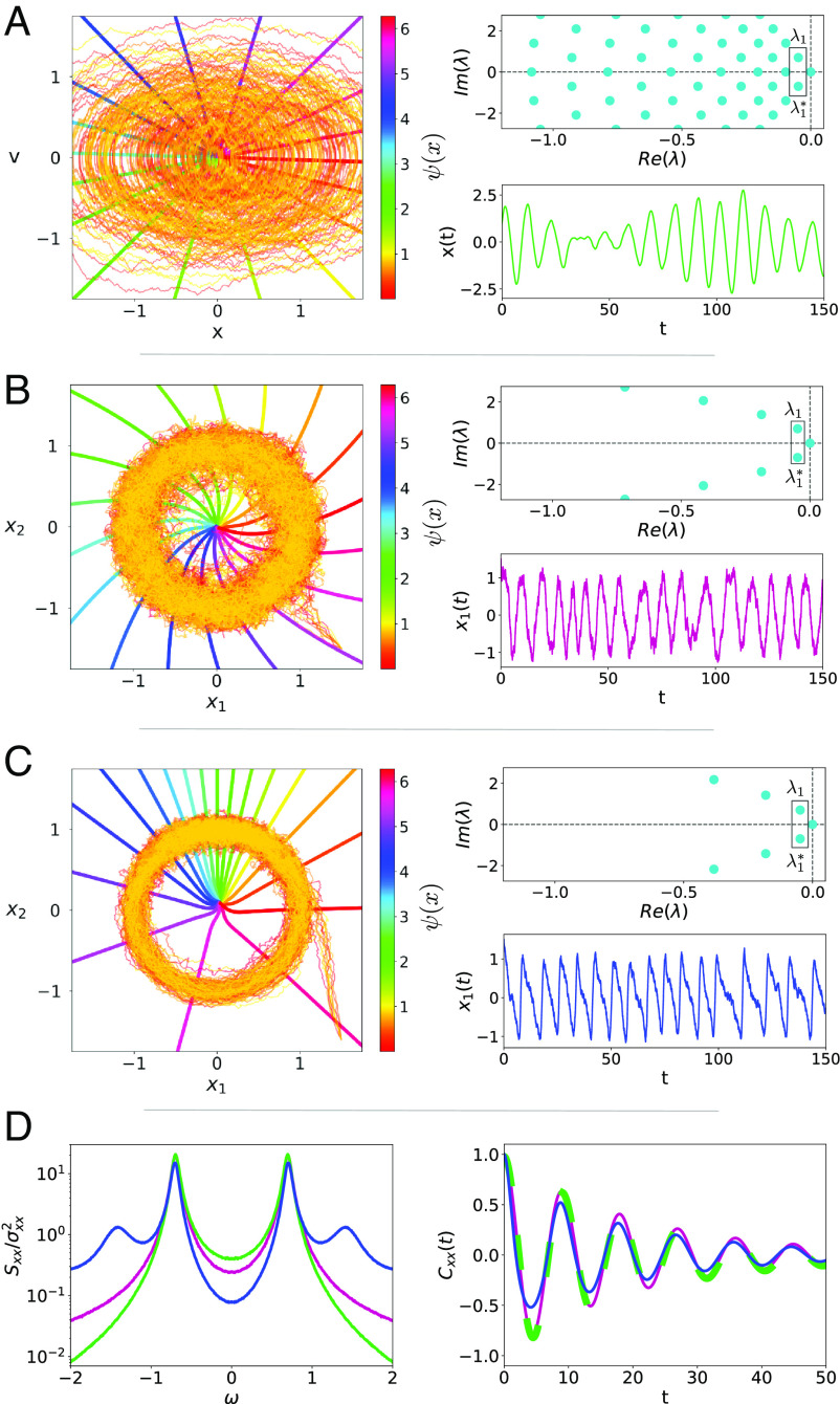
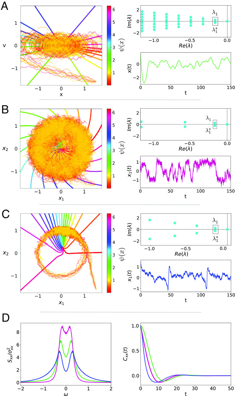
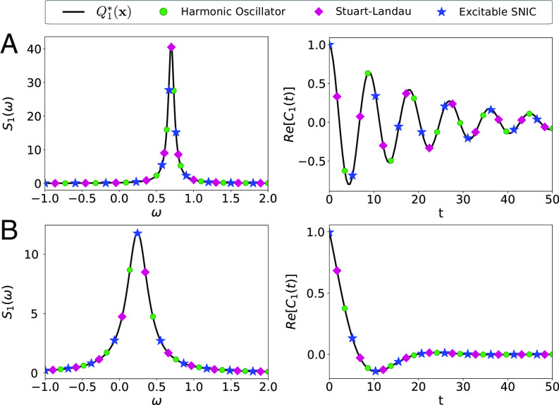
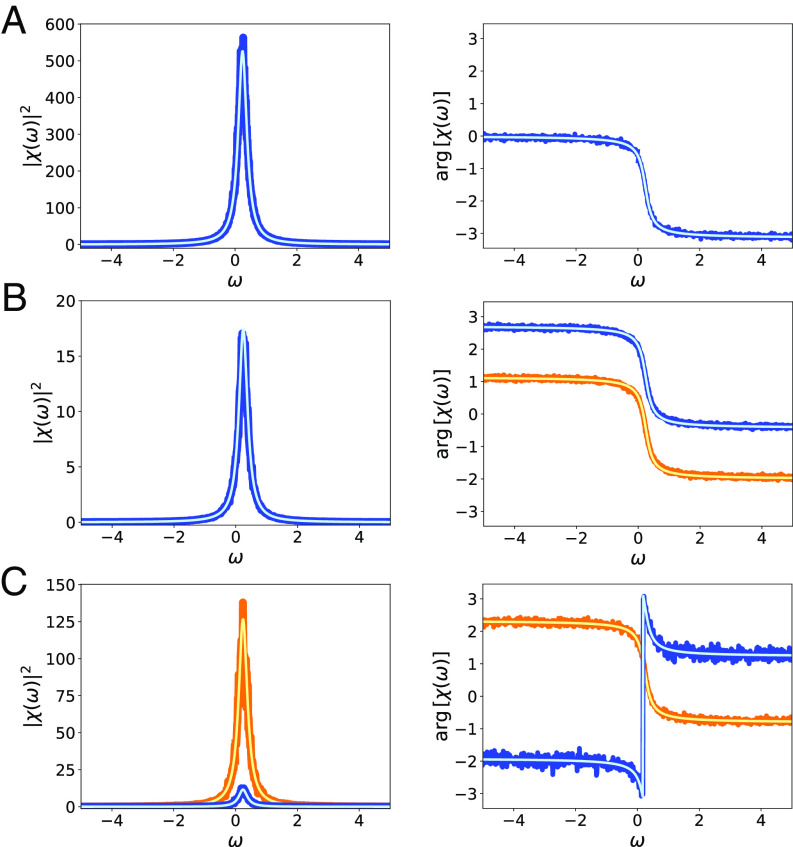
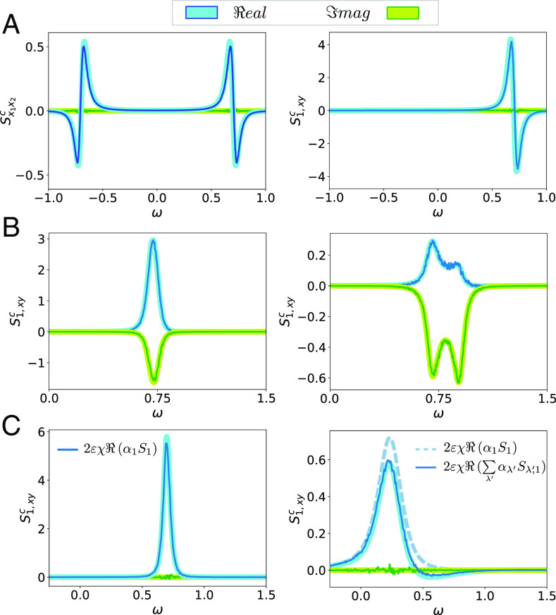
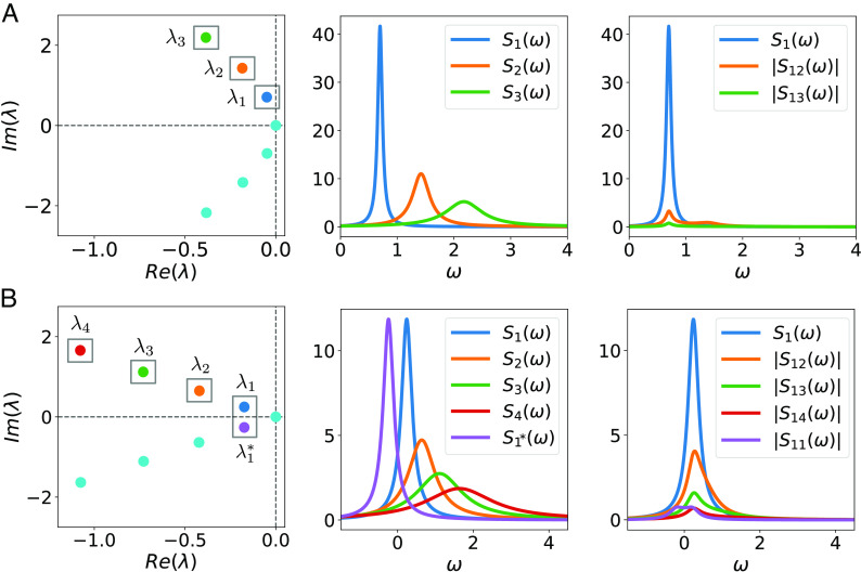
Many systems in physics, chemistry, and biology exhibit oscillations with a pronounced random component. Such stochastic oscillations can emerge via different mechanisms, for example, linear dynamics of a stable focus with fluctuations, limit-cycle systems perturbed by noise, or excitable systems in which random inputs lead to a train of pulses. Despite their diverse origins, the phenomenology of random oscillations can be strikingly similar. Here, we introduce a nonlinear transformation of stochastic oscillators to a complex-valued function [Formula: see text](x) that greatly simplifies and unifies the mathematical description of the oscillator's spontaneous activity, its response to an external time-dependent perturbation, and the correlation statistics of different oscillators that are weakly coupled. The function [Formula: see text] (x) is the eigenfunction of the Kolmogorov backward operator with the least negative (but nonvanishing) eigenvalue λ₁ = μ₁ + iω₁. The resulting power spectrum of the complex-valued function is exactly given by a Lorentz spectrum with peak frequency ω₁ and half-width μ₁; its susceptibility with respect to a weak external forcing is given by a simple one-pole filter, centered around ω₁; and the cross-spectrum between two coupled oscillators can be easily expressed by a combination of the spontaneous power spectra of the uncoupled systems and their susceptibilities. Our approach makes qualitatively different stochastic oscillators comparable, provides simple characteristics for the coherence of the random oscillation, and gives a framework for the description of weakly coupled oscillators.

Keywords: cross-correlation of coupled oscillators; linear response; nonlinear stochastic differential equations; power spectrum.

Fig. 1.

Three models of “robust” stochastic oscillations. In the three panels, we show for each model ten sample trajectories in phase space together with the stochastic asymptotic phase ψ(x) (Left), a time series of one of the components (Lower Right), and the spectrum of eigenvalues (Top Right). For the three models, parameters have been tuned so they have the same value for the eigenvalue λ₁ = −0.048 + 0.698i with the smallest nonvanishing real part. (A) Damped noisy harmonic oscillator for M = 1, γ = 0.096, ω₀ = 0.699, D = 0.01125. (B) Noisy Stuart–Landau for a = 1, b = −0.3, D₁ = D₂ = 0.04. (C) Noisy SNIC model (beyond the bifurcation, i.e., in the limit-cycle regime) for m = 1.216, n = 1.014, and D₁ = D₂ = 0.0119. (D) Power spectra (Left) and correlation function (Right) of x(t) (harmonic oscillator, green), x₁(t) (noisy Stuart–Landau model, purple), and x₁(t) (SNIC model, blue).

Fig. 2.

Three models of stochastic oscillations. In the three panels, we show for each model ten sample trajectories in phase space together with the stochastic asymptotic phase ψ(x) (Left), a time series of one of the components (Lower Right), and the spectrum of eigenvalues (Top Right). For the three models, parameters have been tuned, so they have the same value for slowest decaying eigenvalue λ₁ = −0.168 + 0.241i. (A) Damped noisy harmonic oscillator for M = 1, γ = 0.337, ω₀ = 0.294, D = 0.01125. (B) Noisy Stuart–Landau for a = 1, b = −0.713, and D₁ = D₂ = 0.0995. (C) Noisy SNIC model (prior to the bifurcation, i.e., in the excitable regime) for m = 0.99, n = 1, and D₁ = D₂ = 0.01125. (D) Power spectra (Left) and correlation function (Right) of x(t) (harmonic oscillator, green), x₁(t) (noisy Stuart–Landau model, purple), and x₁(t) (excitable SNIC model, blue).

Fig. 3.

Power spectra S₁(ω) and real part of the autocorrelation function C₁(t) of $Q_1^{*}$ (x(t)) for the different models with parameters in A and B as in Figs. 1 and 2, respectively. (A) For parameters from Fig. 1 (chosen such that λ₁ = μ₁ + iω₁ is approximately the same for all models with μ₁ = −0.048, ω₁ = 0.698, leading to a more coherent oscillation with a quality factor of |ω₁/μ₁|=14.3), we compare Eq. 15 (solid line) to stochastic simulations of the three models (symbols). (B) For parameters from Fig. 2 (chosen such that λ₁ = μ₁ + iω₁ is approximately the same for all models with μ₁ = −0.168, ω₁ = 0.241, leading to a less coherent oscillation with a quality factor of |ω₁/μ₁|=1.43), we compare Eq. 15 (solid line) to stochastic simulations of the three models (symbols).

Fig. 4.

Susceptibility functions χ_e(ω) of the variable $Q_1^{*}$ (x(t)) for the different models with the same parameters as in Fig. 2 and different perturbation vectors e as indicated. For each model, we show the squared of the absolute value, |χ_e(ω)|², (Left) showing a Lorentzian profile and its angle arg(χ_e(ω)) (Right). The perturbation vectors are e₁ = (1, 0)^⊤ and e₂ = (0, 1)^⊤. (A) The harmonic oscillator β_ev = −3.87i (blue, computations; cyan, theory); (B) Stuart–Landau model β_e1 = 0.641 − 0.297i (orange, computations; yellow, theory), β_e2 = 0.297 + 0.641i, (blue, computations; cyan, theory); (C) SNIC excitable system β_e1 = 1.38 + 1.3i (orange, computations; yellow, theory), β_e2 = −0.54 + 0.19i (blue, computations; cyan, theory).

Fig. 5.

Cross-spectra of two coupled units for weak coupling strength ε = 0.01. In all panels, the thin (thick) lines indicate simulations (theory); blue (green) corresponds to real (imaginary) part. (A) For two harmonic oscillators with parameters as in Fig. 1, we show cross-spectra between the position variables of each oscillator (Left) and between the $Q_1^{*}$ functions, $S_{1,\mathbf{\text{yx}}}^c$. (B) For two symmetrically coupled but nonidentical Stuart–Landau oscillators, we show the cross-spectrum between the $Q_1^{*}$ functions; Left: oscillators slightly detuned with one oscillator as in Fig. 1 and the other one with a changed value of b = −0.25; Right: the second oscillator is more strongly detuned with b = −0.1. (C) For two coupled identically SNIC systems, we show the cross-spectra $S_{1,\mathbf{\text{yx}}}^c$ with parameters as in Fig. 1 (Left) and Fig. 2 (Right). In the Right, two versions of the theory are shown: approximations by one mode (dashed line) and by the five leading terms (solid line, see text).

Fig. 6.

Spectral overlap and cross-spectra between $Q_1^{*}$ and the rest of the backward modes for a more (A) and less (B) coherent oscillator. Spectrum of eigenvalues (Left), power spectrum S_λ of different eigenmodes (Mid), and the cross-spectra between $Q_1^{*}$ and different eigenmodes (Right). SNIC model with parameters in A and B as in Figs. 1 and 2, respectively.

References

1. Potoyan D. A., Wolynes P. G., On the dephasing of genetic oscillators. Proc. Natl. Acad. Sci. U.S.A. 111, 2391–2396 (2014). - PMC - PubMed
1. Lugo C. A., McKane A. J., Quasicycles in a spatial predator–prey model. Phys. Rev. E 78, 051911 (2008). - PubMed
1. Rubin J. E., Earn D. J., Greenwood P. E., Parsons T. L., Abbott K. C., Irregular population cycles driven by environmental stochasticity and saddle crawlbys. Oikos 2023, e09290 (2023).
1. Dubbeldam J. L. A., Krauskopf B., Lenstra D., Excitability and coherence resonance in lasers with saturable absorber. Phys. Rev. E 60, 6580 (1999). - PubMed
1. García-Ojalvo J., Casademont J., Torrent M. C., Coherence and synchronization in diode-laser arrays with delayed global coupling. Int. J. Bifurcat. Chaos 9, 2225 (1999).