Predicting scale-dependent chromatin polymer properties from systematic coarse-graining

Abstract

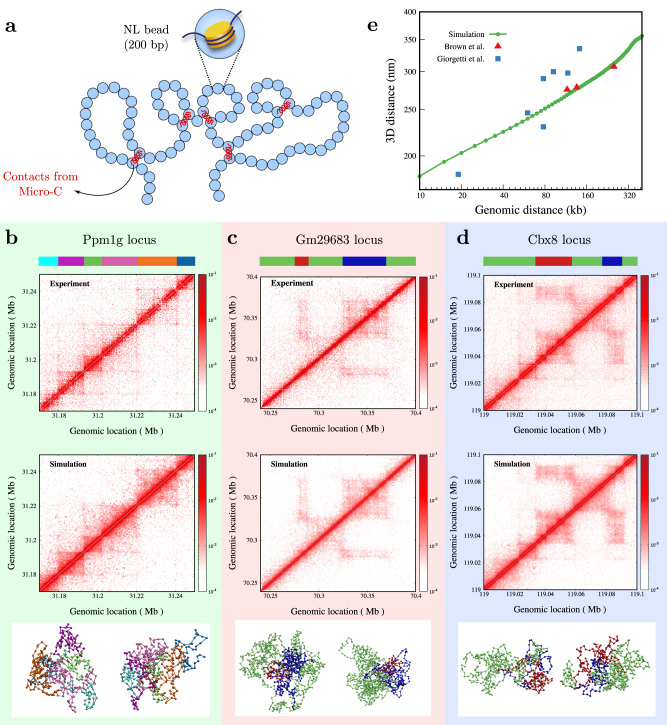
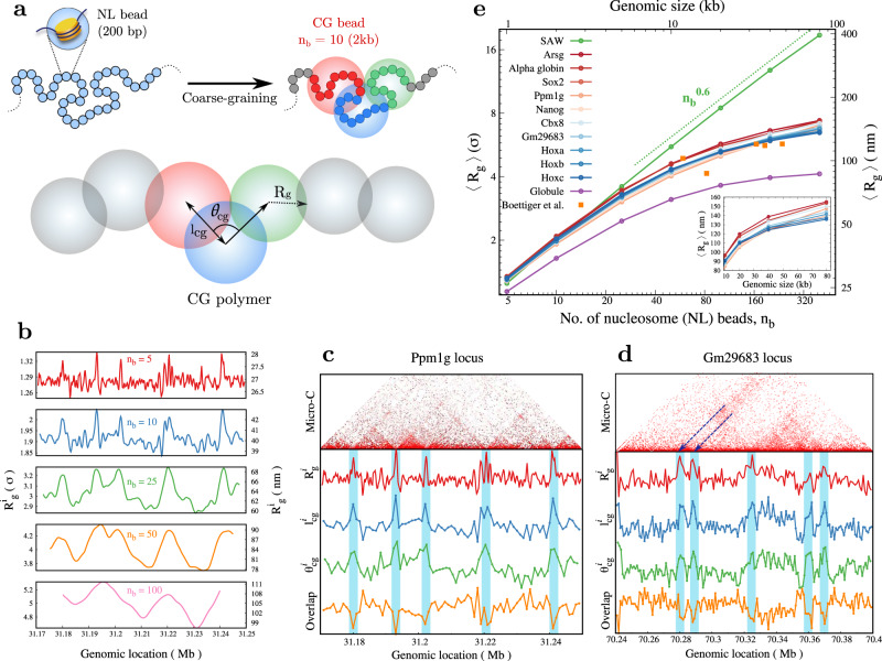
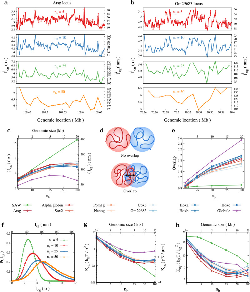
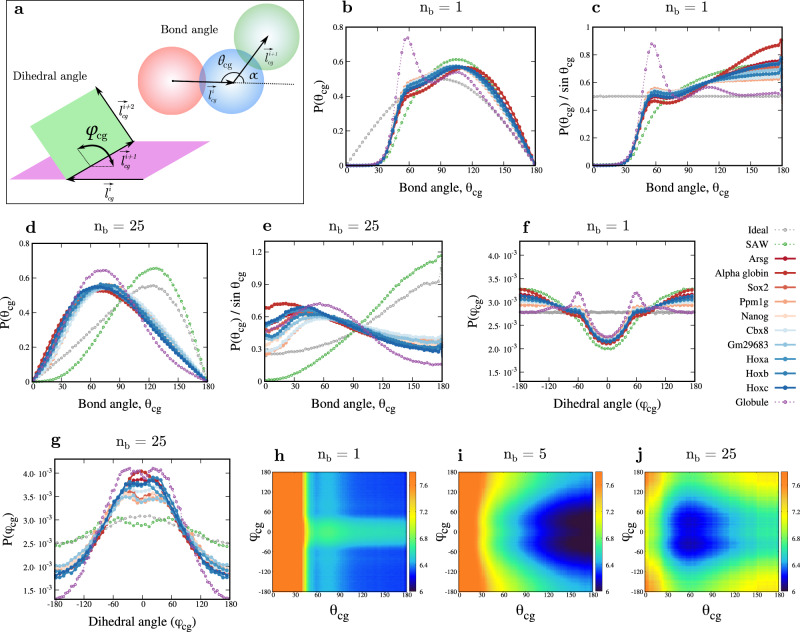
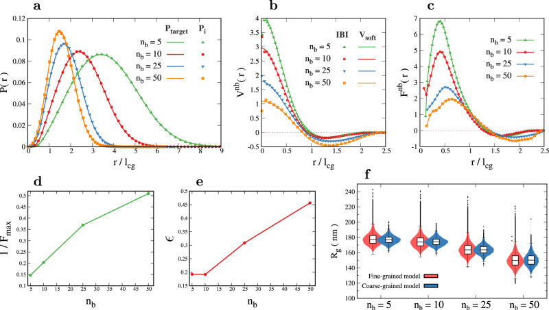
Simulating chromatin is crucial for predicting genome organization and dynamics. Although coarse-grained bead-spring polymer models are commonly used to describe chromatin, the relevant bead dimensions, elastic properties, and the nature of inter-bead potentials are unknown. Using nucleosome-resolution contact probability (Micro-C) data, we systematically coarse-grain chromatin and predict quantities essential for polymer representation of chromatin. We compute size distributions of chromatin beads for different coarse-graining scales, quantify fluctuations and distributions of bond lengths between neighboring regions, and derive effective spring constant values. Unlike the prevalent notion, our findings argue that coarse-grained chromatin beads must be considered as soft particles that can overlap, and we derive an effective inter-bead soft potential and quantify an overlap parameter. We also compute angle distributions giving insights into intrinsic folding and local bendability of chromatin. While the nucleosome-linker DNA bond angle naturally emerges from our work, we show two populations of local structural states. The bead sizes, bond lengths, and bond angles show different mean behavior at Topologically Associating Domain (TAD) boundaries and TAD interiors. We integrate our findings into a coarse-grained polymer model and provide quantitative estimates of all model parameters, which can serve as a foundational basis for all future coarse-grained chromatin simulations.

Fig. 1. Chromatin configurations are consistent with experiments.

a Schematic of the fine-grained chromatin polymer with one bead representing 200 bp nucleosome+linker (NL) chromatin. An ensemble of configurations is generated such that any pair of beads (i, j) is connected (red springs) with a probability p_ij, based on observed contacts in Micro-C experiments by Hsieh et al. (see text). b–d Comparison of contact maps obtained from our simulation to experiments for a euchromatic region (b Ppm1g locus) and two heterochromatic regions (c Gm29683 locus, and d Cbx8 locus). The bottom panel shows representative snapshots from the simulations, where the bead colors represent different domains, as shown in the color strip at the top. e 3D distance from our alpha globin simulation (green filled circles) compared with available experimental data for the same region (red filled triangles) taken from Brown et al., and other regions (blue squares) of similar genomic length range taken from Giorgetti et al.. Source data are provided as a Source Data file.

Fig. 2. Coarse-graining, bead size and its variability along the genome.

a Schematic showing the coarse-graining procedure and quantities of interest. The fine-grained polymer of N beads (small beads, representing 200 bp of nucleosome+linker (NL)) is coarse-grained into N_cg big beads, with each big coarse-grained bead containing n_b = N/N_cg beads. For illustration purposes, ten small colored beads (n_b = 10) are coarse-grained into one big CG bead. l_cg is the length of the bond connecting two successive coarse-grained beads, θ_cg is the angle between two successive bonds, and R_g is the radius of gyration of the coarse-grained polymer segment of size n_b. b Average radius of gyration at different genomic locations ($R_g^i$) for different n_b values for the Ppm1g locus. c–d Variation of $R_g^i$ and other quantities ($l_{cg}^i$, ${\theta }_{cg}^i$, and overlap, see text) along the chromatin contour (n_b = 5) for (c) a euchromatic Ppm1g locus and (d) a heterochromatic Gm29683 locus. Note different behavior at the domain boundaries. e Mean R_g for different coarse-graining sizes (n_b) showing the predicted range of values for different chromatin states. The chromatin loci with broad euchromatic characteristics are plotted in shades of red, while the loci with broad heterochromatic marks are plotted using shades of blue. Experimental data from Boettiger et al. is added (orange squares; repressed chromatin domains in Drosophila cells) to demonstrate that the predicted R_g values are reasonable. The dotted line is shown as a guide to the eye. R_g values are presented in the units of NL bead size σ (Y₁ axis) and also in nm (Y₂ axis). Source data are provided as a Source Data file.

Fig. 3. Chromatin as bead-spring chain: bond length, spring constant and overlap.

a, b Spatial variation of average bond length ($l_{cg}^i$) for (a) euchromatic Arsg locus and (b) heterochromatic Gm29683 locus is plotted for different coarse-graining sizes (n_b). c Average l_cg for different coarse-graining sizes showing the range of values possible from SAW to globule; presented in two different units in Y₁ and Y₂ axes. d Schematic showing two nearby long polymer segments “mixing” (or not mixing) in 3D space resulting in overlap (or no overlap) of coarse-grained (colored) beads. e A parameter that quantifies the extent of overlap is plotted for different n_b values. f Distribution of l_cg for euchromatin region. g, h The effective spring constant (K_cg) quantifies the fluctuation between neighboring coarse-grained beads for chromatin segments in different epigenetic states, presented in two different units. CG simulations would need units in (h). Source data are provided as a Source Data file.

Fig. 4. Angle distributions of chromatin segments revealing bendability.

a Schematic showing the bond angle θ_cg and dihedral angle ϕ_cg between coarse-grained beads. b, c Distribution of angles for different chromatin loci, for the fine-grained model (n_b = 1) with nucleosome-linker (200 bp) resolution (b) P(θ_cg), and (c) the distribution with a different measure P(θ_cg)/$\sin$(θ_cg) are shown. d, e Similar angle distribution for the coarse-grained chromatin model with one bead representing 5 kb (n_b = 25) of chromatin is shown in (d) P(θ_cg) and (e) P(θ_cg)/$\sin$(θ_cg). f, g The distribution of dihedral angles for different chromatin loci for (f) the fine-grained model (n_b = 1) and (g) coarse-grained chromatin with one bead representing 5 kb (n_b = 25) of chromatin. h–j (θ_cg- ϕ_cg) energy plot for the Ppm1g locus for (h) the fine-grained model (n_b = 1), (i) CG chromatin with one bead representing 1 kb chromatin (n_b = 5) and (j) CG chromatin with one bead representing 5 kb chromatin (n_b = 25). Source data are provided as a Source Data file.

Fig. 5. Soft inter-bead potential energy for coarse-grained chromatin beads.

a The distribution of distances between all non-bonded beads obtained from the iterative Boltzmann inversion (IBI) method after convergence P_i(r) (points) matches well with the fine-grained chromatin target distribution P_target(r) (solid lines) for appropriate levels of coarse-graining. b The non-bonded potential (V^nb) obtained from the IBI method (points) and the functional form for the soft potential V_soft(r) (solid lines using Eq. (2); see parameters in Supplementary Table 2) for different values of n_b. c The force derived from the potential in (c) for different values of n_b. d The inverse of the maximum value of the force as a function of n_b as a measure of softness. e The depth (ϵ) of the V^nb potential is plotted as a function of coarse-graining size. f The radius of gyration measured from the coarse-grained simulation with soft potential is compared with the R_g from the fine-grained model for corresponding levels of coarse-graining. The violin plots show the distribution of data and the box plots on top depict the 25–75th percentiles, with the middle line denoting the median. The whiskers extend to 1.5 times the interquartile range, and outliers are indicated with dots. n = 60,000 independent sample polymer configurations were used in fine-grained model while n = 5000 independent sample polymer configurations were used in coarse-grained model for all values of n_b. Source data are provided as a Source Data file.

References

1. Alberts, B. Molecular Biology of The Cell, 6th edn (Garland Science, Taylor and Francis Group, New York, 2014).
1. Bickmore WA. The spatial organization of the human genome. Annu. Rev. Genomics Hum. Genet. 2013;14:67–84. doi: 10.1146/annurev-genom-091212-153515. - DOI - PubMed
1. Kornberg RD, Lorch Y. Twenty-five years of the nucleosome, fundamental particle of the eukaryote chromosome. Cell. 1999;98:285–294. doi: 10.1016/S0092-8674(00)81958-3. - DOI - PubMed
1. Rowley MJ, Corces VG. Organizational principles of 3D genome architecture. Nat. Rev. Genet. 2018;19:1. doi: 10.1038/s41576-018-0060-8. - DOI - PMC - PubMed
1. Hug CB, Vaquerizas JM. The birth of the 3d genome during early embryonic development. Trends Genet. 2018;34:903–914. doi: 10.1016/j.tig.2018.09.002. - DOI - PubMed
Publication types