

A fast phenotype approach of 3D point clouds of Pinus massoniana seedlings
- PMID: 37434607
- PMCID: PMC10332475
- DOI: 10.3389/fpls.2023.1146490
A fast phenotype approach of 3D point clouds of Pinus massoniana seedlings
Abstract
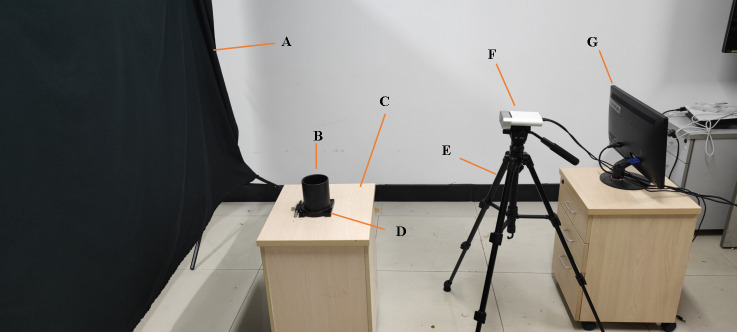
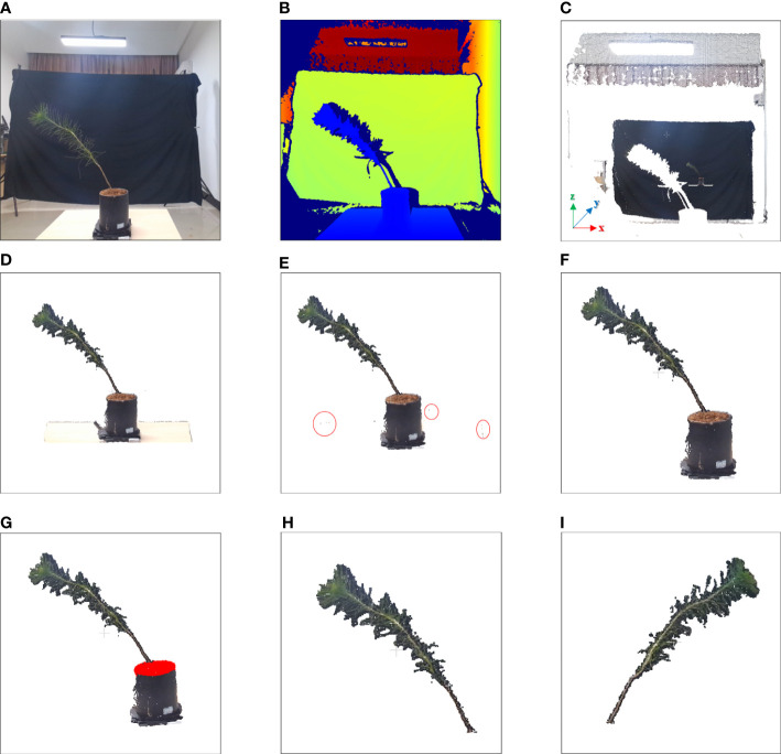
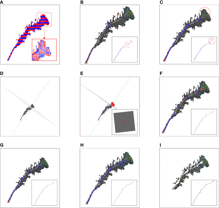
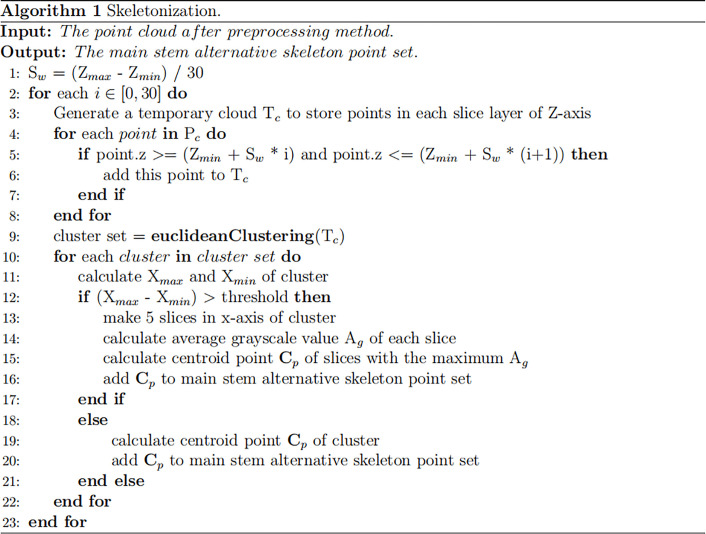
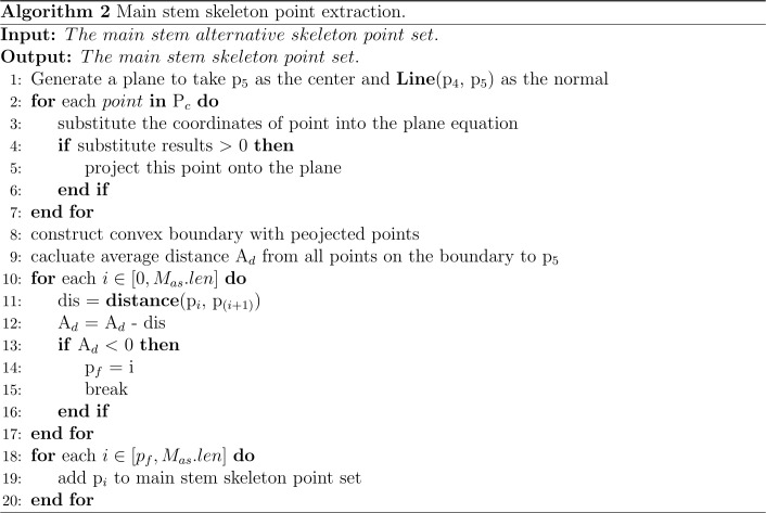
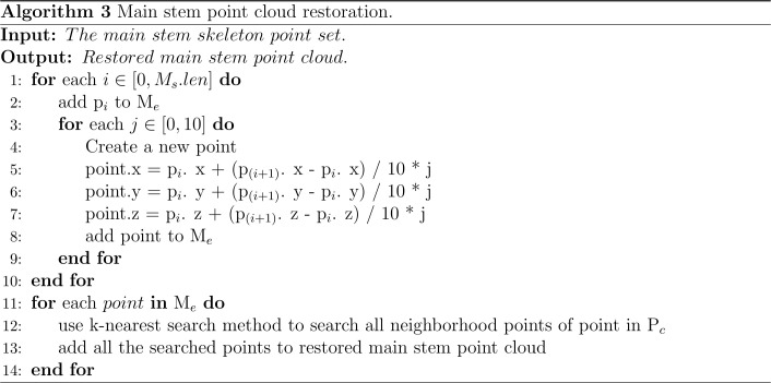
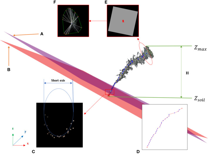
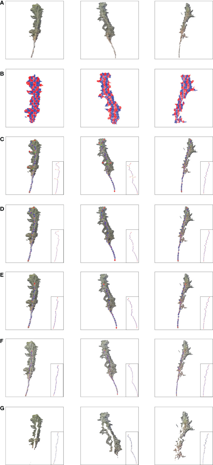
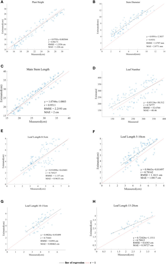
The phenotyping of Pinus massoniana seedlings is essential for breeding, vegetation protection, resource investigation, and so on. Few reports regarding estimating phenotypic parameters accurately in the seeding stage of Pinus massoniana plants using 3D point clouds exist. In this study, seedlings with heights of approximately 15-30 cm were taken as the research object, and an improved approach was proposed to automatically calculate five key parameters. The key procedure of our proposed method includes point cloud preprocessing, stem and leaf segmentation, and morphological trait extraction steps. In the skeletonization step, the cloud points were sliced in vertical and horizontal directions, gray value clustering was performed, the centroid of the slice was regarded as the skeleton point, and the alternative skeleton point of the main stem was determined by the DAG single source shortest path algorithm. Then, the skeleton points of the canopy in the alternative skeleton point were removed, and the skeleton point of the main stem was obtained. Last, the main stem skeleton point after linear interpolation was restored, while stem and leaf segmentation was achieved. Because of the leaf morphological characteristics of Pinus massoniana, its leaves are large and dense. Even using a high-precision industrial digital readout, it is impossible to obtain a 3D model of Pinus massoniana leaves. In this study, an improved algorithm based on density and projection is proposed to estimate the relevant parameters of Pinus massoniana leaves. Finally, five important phenotypic parameters, namely plant height, stem diameter, main stem length, regional leaf length, and total leaf number, are obtained from the skeleton and the point cloud after separation and reconstruction. The experimental results showed that there was a high correlation between the actual value from manual measurement and the predicted value from the algorithm output. The accuracies of the main stem diameter, main stem length, and leaf length were 93.5%, 95.7%, and 83.8%, respectively, which meet the requirements of real applications.
Keywords: 3D point cloud; Pinus massoniana seedlings; phenotyping; skeletonization; slicing.
Copyright © 2023 Zhou, Zhou, Long, Wang, Zhou and Chen.
Conflict of interest statement
The authors declare that the research was conducted in the absence of any commercial or financial relationships that could be construed as a potential conflict of interest.
Figures
Similar articles
-
An automated phenotyping method for Chinese Cymbidium seedlings based on 3D point cloud.Plant Methods. 2024 Sep 30;20(1):151. doi: 10.1186/s13007-024-01277-1. Plant Methods. 2024. PMID: 39343899 Free PMC article.
-
An Accurate Skeleton Extraction Approach From 3D Point Clouds of Maize Plants.Front Plant Sci. 2019 Mar 7;10:248. doi: 10.3389/fpls.2019.00248. eCollection 2019. Front Plant Sci. 2019. PMID: 30899271 Free PMC article.
-
Automatic Branch-Leaf Segmentation and Leaf Phenotypic Parameter Estimation of Pear Trees Based on Three-Dimensional Point Clouds.Sensors (Basel). 2023 May 8;23(9):4572. doi: 10.3390/s23094572. Sensors (Basel). 2023. PMID: 37177776 Free PMC article.
-
Measurement of Maize Leaf Phenotypic Parameters Based on 3D Point Cloud.Sensors (Basel). 2025 Apr 30;25(9):2854. doi: 10.3390/s25092854. Sensors (Basel). 2025. PMID: 40363288 Free PMC article.
-
Measuring crops in 3D: using geometry for plant phenotyping.Plant Methods. 2019 Sep 3;15:103. doi: 10.1186/s13007-019-0490-0. eCollection 2019. Plant Methods. 2019. PMID: 31497064 Free PMC article. Review.
Cited by
-
An automated phenotyping method for Chinese Cymbidium seedlings based on 3D point cloud.Plant Methods. 2024 Sep 30;20(1):151. doi: 10.1186/s13007-024-01277-1. Plant Methods. 2024. PMID: 39343899 Free PMC article.
References
-
- Besl P. J., Jain R. C. (1988). Segmentation through variable-order surface fitting. IEEE Trans. Pattern Anal. Mach. Intell. 10 (2), 167–192. doi: 10.1109/34.3881 - DOI
-
- Bradski G., Kaehler A. (2008). Learning OpenCV: computer vision with the OpenCV library (O'Reilly Media, Inc; ). https://ieeexplore.ieee.org/document/5233425/
-
- Cao J., Tagliasacchi A., Olson M., Zhang H., Su Z. (2010). “Point cloud skeletons via laplacian based contraction,” in 2010 Shape Modeling International Conference. 187–197. doi: 10.1109/SMI.2010.25 - DOI
-
- Cupec R., Vidović I., Filko D., Đurović P. (2020). Object recognition based on convex hull alignment. Pattern Recognit. 102, 107199. doi: 10.1016/j.patcog.2020.107199 - DOI
-
- Dalitz C., Schramke T., Jeltsch M. (2017). Iterative hough transform for line detection in 3D point clouds. Image Process. On Line 7, 184–196. doi: 10.5201/ipol.2017.208 - DOI
LinkOut - more resources
Full Text Sources