Surface and subsurface oceanographic features drive forage fish distributions and aggregations: Implications for prey availability to top predators in the US Northeast Shelf ecosystem

Abstract

Forage fishes are a critical food web link in marine ecosystems, aggregating in a hierarchical patch structure over multiple spatial and temporal scales. Surface-level forage fish aggregations (FFAs) represent a concentrated source of prey available to surface- and shallow-foraging marine predators. Existing survey and analysis methods are often imperfect for studying forage fishes at scales appropriate to foraging predators, making it difficult to quantify predator-prey interactions. In many cases, general distributions of forage fish species are known; however, these may not represent surface-level prey availability to predators. Likewise, we lack an understanding of the oceanographic drivers of spatial patterns of prey aggregation and availability or forage fish community patterns. Specifically, we applied Bayesian joint species distribution models to bottom trawl survey data to assess species- and community-level forage fish distribution patterns across the US Northeast Continental Shelf (NES) ecosystem. Aerial digital surveys gathered data on surface FFAs at two project sites within the NES, which we used in a spatially explicit hierarchical Bayesian model to estimate the abundance and size of surface FFAs. We used these models to examine the oceanographic drivers of forage fish distributions and aggregations. Our results suggest that, in the NES, regions of high community species richness are spatially consistent with regions of high surface FFA abundance. Bathymetric depth drove both patterns, while subsurface features, such as mixed layer depth, primarily influenced aggregation behavior and surface features, such as sea surface temperature, sub-mesoscale eddies, and fronts influenced forage fish diversity. In combination, these models help quantify the availability of forage fishes to marine predators and represent a novel application of spatial models to aerial digital survey data.

Keywords: forage fish aggregation; hierarchical Bayesian model; joint species distribution model; predator–prey interactions; trophodynamics.

FIGURE 1

(a) US Northeast Continental Shelf (NES) study area, (b) New York (NY) Bight aerial digital survey transects, and (c) Mid‐Atlantic Bight aerial digital survey transects. Model prediction extents are depicted via blue (NES) and orange (FFA) outlines. Relevant geographic features are labeled (see legend). FFA, forage fish aggregation; ME, Maine; OPA, offshore planning area; WEA, wind energy area.

FIGURE 2

Beta parameter estimates for the (a) autumn and (b) spring community models. Orange and blue grid squares represent a significant relationship (either positive or negative, respectively) between the probability of occupancy and each environmental covariate. White grid cells represent non‐significant relationships. Beta parameters were considered significant if they had at least 95% posterior support. The top panels depict the community‐level covariate effect size, calculated as the mean absolute parameter values.

FIGURE 3

(a) Beta parameter estimates and credible intervals (CIs) from the forage fish aggregation (FFA) abundance model. Gray points represent the parameter medians, thick lines the 50% CI, and thin lines the 95% CI. Parameters with gray CIs are not significant. (b–f) FFA abundance predictions relative to the five strongest beta parameters. Shaded areas represent the 95% CI of the estimate.

FIGURE 4

(a) Beta parameter estimates and credible intervals (CI) from the forage fish aggregation (FFA) size model. Points represent the parameter medians, thick lines the 50% CI, and thin lines the 95% CI. The inset (gray box) enlarges the scale for parameters close to zero to improve readability. Parameters with gray CIs are not significant. (b–d) FFA size predictions relative to the three strongest beta parameters. Shaded areas represent the 95% CI of the estimate.

FIGURE 5

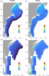
Forage fish community species richness for (a, c) autumn and (b, d) spring across the Northeast Continental Shelf (NES) study area. Black outlines (a, b) delineate the forage fish aggregation (FFA) study area. The bottom panels enlarge the FFA study area. Species richness was calculated as the summed probability of occurrence across all species. Note that the scales for autumn and spring differ due to differences in the maximum species richness possible for each season.

FIGURE 6

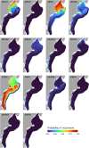
Autumn community model predictions of forage fish occurrence, based on bottom trawl data. Species codes are defined in Table 1.

FIGURE 7

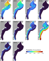
Spring community model predictions of forage fish occurrence, based on bottom trawl data. Species codes are defined in Table 1.

FIGURE 8

Predicted spatial distribution of forage fish aggregation (FFA) abundance, size, and surface availability (abundance × size, cumulative m²). The spatial extent of the size and availability predictions has been reduced to only include on‐shelf areas.

FIGURE 9

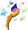
Autumn forage fish community types: six distinct forage fish community types were identified across the NES study area via k‐means cluster analysis. Circular bar plots depict the prevalence (i.e., mean occurrence probability) of species within the community type (y‐scale max = 1). Species codes are defined in Table 1. Species with a prevalence <0.003 are not shown. Black outlines define the forage fish aggregation (FFA) study area. See Appendix 2: Table A3a for prevalence estimations. NES – U.S. Northeast Continental Shelf.

FIGURE 10

Spring forage fish community types: six distinct community types were identified across the NES study area via k‐means cluster analysis. Circular bar plots depict the prevalence (i.e., mean occurrence probability) of species within the community type (y‐scale max = 1). Species codes are defined in Table 1. Species with a prevalence <0.003 are not shown. Black outlines define the forage fish aggregation study area. See Appendix 2: Table A3b for prevalence estimations. NES – U.S. Northeast Continental Shelf.

FIGURE A1

Potential scale reduction factors (PSRFs) and effective sample size (ESS) for monitored parameters to evaluate autumn (a, c) and spring (b, d) HMSC model convergence for the best fitting Fprob models. For the PSRF values, the autumn model had 96.6%, and the spring model had 82.4% below 1.1 (red dashed line). The 0.95 quantiles for PSRF were 1.06 and 1.26 for autumn and spring, respectively. The ESS values of all parameters for both models are above 400 (red dashed line).

FIGURE A2

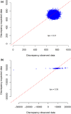
Posterior predictive check for (a) abundance and (b) size forage fish aggregation models, showing the observed versus expected Chi‐square discrepancy measures (Freeman–Tukey goodness‐of‐fit) and the calculated Bayesian p‐values (bpv).

FIGURE A3

Residual species‐to‐species associations (i.e., species which co‐occur more or less than expected based on species' niches) in the (a, b) autumn and (c, d) spring community models. Panels (a) and (c) are due to the temporal random effect, while panels (b) and (d) are due to the tow random effect. Orange and blue indicate species pairs with at least 0.95 posterior support for a positive or negative association, respectively. The intensity of color and size of the marker indicates the strength of the association (in units of correlation). Species codes are defined in Table 1.

References

1. Abrahms, B. , Scales, K. L. , Hazen, E. L. , Bograd, S. J. , Schick, R. S. , Robinson, P. W. , & Costa, D. P. (2018). Mesoscale activity facilitates energy gain in a top predator. Proceedings of the Royal Society B: Biological Sciences, 285(1885), 20181101. 10.1098/rspb.2018.1101 - DOI - PMC - PubMed
1. Arimitsu, M. L. , Piatt, J. F. , Hatch, S. , Suryan, R. M. , Batten, S. , Bishop, M. A. , Campbell, R. W. , Coletti, H. , Cushing, D. , Gorman, K. , Hopcroft, R. R. , Kuletz, K. J. , Marsteller, C. , McKinstry, C. , McGowan, D. , Moran, J. , Pegau, S. , Schaefer, A. , Schoen, S. , … von Biela, V. R. (2021). Heatwave‐induced synchrony within forage fish portfolio disrupts energy flow to top pelagic predators. Global Change Biology, 27(9), 1859–1878. 10.1111/gcb.15556 - DOI - PMC - PubMed
1. Arkema, K. K. , Abramson, S. C. , & Dewsbury, B. M. (2006). Marine ecosystem‐based management: From characterization to implementation. Ecology and Environment, 4(10), 525–532.
1. Banerjee, S. , Carlin, B. P. , Gelfand, A. E. , & Banerjee, S. (2003). Hierarchical modeling and analysis for spatial data, hierarchical modeling and analysis for spatial data. Chapman and Hall/CRC. 10.1201/9780203487808 - DOI
1. Bangley, C. W. , Curtis, T. H. , Secor, D. H. , Latour, R. J. , & Ogburn, M. B. (2020). Identifying important juvenile dusky shark habitat in the Northwest Atlantic Ocean using acoustic telemetry and spatial modeling. Marine and Coastal Fisheries, 12(5), 348–363. 10.1002/MCF2.10120 - DOI
LinkOut - more resources