Mass Spectrometry-Based Evaluation of the Bland-Altman Approach: Review, Discussion, and Proposal

Abstract

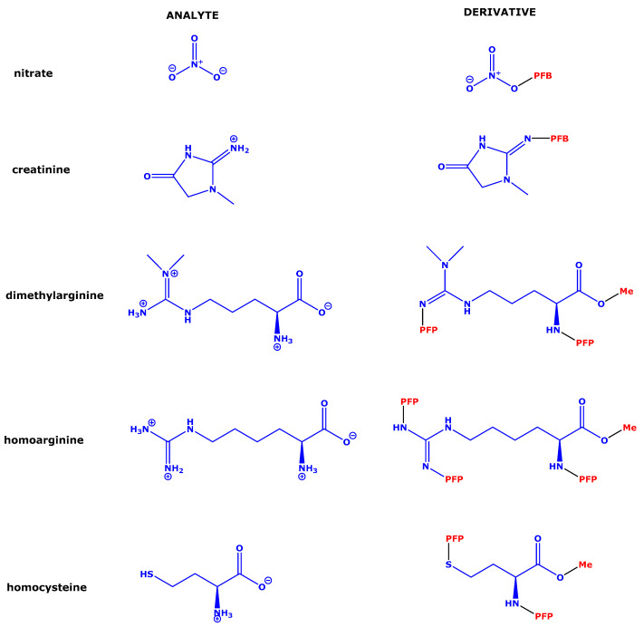
Reliable quantification in biological systems of endogenous low- and high-molecular substances, drugs and their metabolites, is of particular importance in diagnosis and therapy, and in basic and clinical research. The analytical characteristics of analytical approaches have many differences, including in core features such as accuracy, precision, specificity, and limits of detection (LOD) and quantitation (LOQ). Several different mathematic approaches were developed and used for the comparison of two analytical methods applied to the same chemical compound in the same biological sample. Generally, comparisons of results obtained by two analytical methods yields different quantitative results. Yet, which mathematical approach gives the most reliable results? Which mathematical approach is best suited to demonstrate agreement between the methods, or the superiority of an analytical method A over analytical method B? The simplest and most frequently used method of comparison is the linear regression analysis of data observed by method A (y) and the data observed by method B (x): y = α + βx. In 1986, Bland and Altman indicated that linear regression analysis, notably the use of the correlation coefficient, is inappropriate for method-comparison. Instead, Bland and Altman have suggested an alternative approach, which is generally known as the Bland-Altman approach. Originally, this method of comparison was applied in medicine, for instance, to measure blood pressure by two devices. The Bland-Altman approach was rapidly adapted in analytical chemistry and in clinical chemistry. To date, the approach suggested by Bland-Altman approach is one of the most widely used mathematical approaches for method-comparison. With about 37,000 citations, the original paper published in the journal The Lancet in 1986 is among the most frequently cited scientific papers in this area to date. Nevertheless, the Bland-Altman approach has not been really set on a quantitative basis. No criteria have been proposed thus far, in which the Bland-Altman approach can form the basis on which analytical agreement or the better analytical method can be demonstrated. In this article, the Bland-Altman approach is re-valuated from a quantitative bioanalytical perspective, and an attempt is made to propose acceptance criteria. For this purpose, different analytical methods were compared with Gold Standard analytical methods based on mass spectrometry (MS) and tandem mass spectrometry (MS/MS), i.e., GC-MS, GC-MS/MS, LC-MS and LC-MS/MS. Other chromatographic and non-chromatographic methods were also considered. The results for several different endogenous substances, including nitrate, anandamide, homoarginine, creatinine and malondialdehyde in human plasma, serum and urine are discussed. In addition to the Bland-Altman approach, linear regression analysis and the Oldham-Eksborg method-comparison approaches were used and compared. Special emphasis was given to the relation of difference and mean in the Bland-Altman approach. Currently available guidelines for method validation were also considered. Acceptance criteria for method agreement were proposed, including the slope and correlation coefficient in linear regression, and the coefficient of variation for the percentage difference in the Bland-Altman and Oldham-Eksborg approaches.

Keywords: Bland and Altman approach; Eksborg; Oldham; agreement; biomarkers; comparison; linear regression analysis; mass spectrometry; tandem mass spectrometry; validation.

Scheme 1

Chemical structures of the native analytes (left) and their chemical derivatives (right) discussed in the present work. Nitrate, nitrite, malondialdehyde, and creatinine are derivatized with pentafluorobenzyl bromide in aqueous acetone (e.g., 60 min at 50 °C). Asymmetric dimethylarginine (ADMA), homoarginine and homocysteine are first methylated in 2 M HCl in methanol (e.g., 30 min at 80 °C), and then by pentafluoropropionic anhydride in ethyl acetate (e.g., 60 min at 65 °C). Me, methyl; PFB, Pentafluorobenzyl; PFP, pentafluoropropionyl.

Figure 1

Measurement of nitrate in human urine by GC-MS (i.e., MS, method (1) and GC-MS/MS (i.e., MS/MS, method (2) and their comparison by: (A) linear regression; (B) Bland–Altman; and (C) Oldham–Eksborg. This Figure was constructed by using the data of Table 1 of the article [58]. Samples were analyzed on the instrument TSQ 7000 first by GC-MS in the SIM mode and subsequently by GC-MS/MS in the SRM mode. The closed points in (A) indicate the 95% confidence bands. Horizontal solid lines in (B) indicate the 95% limits of agreement (±1.96 × SD).

Figure 2

Comparison of measurements of asymmetric dimethylarginine (ADMA) in human plasma (method 1) and serum (method 2) of one patient with acute renal failure before, during and after extended haemodialysis for 8 h: (A) linear regression analysis; (B) Bland–Altman; and (C) Oldham–Eksborg. This Figure was constructed by using the data of Table 1 of a previous article [62]. Samples were analyzed for ADMA on the instrument TSQ 7000 by GC-MS/MS in the SRM mode as reported elsewhere [63]. Horizontal solid lines in (B) indicate the 95% limits of agreement.

Figure 3

Comparison of measurements of anandamide (AEA) in 277 human plasma samples by LC-MS/MS (method 1) and by GC-MS/MS (method 2): (A) linear regression analysis; (B) Bland–Altman; and (C) Oldham–Eksborg. Samples were analyzed for AEA on the instrument TSQ 7000 by GC-MS/MS [68] and by Xevo LC-MS/MS [69] as reported in these references. Horizontal solid lines in (B) indicate the 95% limits of agreement.

Figure 3

Comparison of measurements of anandamide (AEA) in 277 human plasma samples by LC-MS/MS (method 1) and by GC-MS/MS (method 2): (A) linear regression analysis; (B) Bland–Altman; and (C) Oldham–Eksborg. Samples were analyzed for AEA on the instrument TSQ 7000 by GC-MS/MS [68] and by Xevo LC-MS/MS [69] as reported in these references. Horizontal solid lines in (B) indicate the 95% limits of agreement.

Figure 4

Comparison of measurements of homoarginine (hArg) in plasma by GC-MS (method 1) and by GC-MS/MS (method 2) in 369 plasma samples of pregnant women: (A) linear regression analysis; (B1,B2) Bland–Altman; and (C) Oldham–Eksborg. Within (B1,B2): linear regression analysis between percentage difference and average. This Figure was constructed by using the data published in a previous article [70]. Note that two different apparatus were used: Samples were analyzed for hArg on the instrument TSQ 7000 by GC-MS/MS in the SRM mode and on the instrument DSQ in the SIM mode as reported elsewhere [70]. Horizontal solid lines in (B1) indicate the 95% limits of agreement. Note that the difference between the methods is used in percentages ((B1), %) and in absolute concentrations ((B2), µM).

Figure 5

Comparison of measurements of homoarginine (hArg) in mouse plasma by GC-MS/MS (method A) and by LC-MS/MS (method B) in 79 plasma samples: (A) linear regression analysis; (B1,B2) Bland–Altman; and (C) Oldham–Eksborg. Within (B1,B2): linear regression analysis between percentage difference and average. This Figure was constructed by using the data published in a previous article [71]. Note that two different apparatus were used: Samples were analyzed for hArg on the instrument TSQ 7000 by GC-MS/MS in the SRM mode and on the instrument Varian 1200 L Triple Quadrupole MS in the SRM mode as reported elsewhere [71]. Horizontal solid lines in (B1,B2) indicate the 95% limits of agreement. Shaded insets indicate ranges of maximum disagreement.

Figure 6

This Figure was constructed by using the data of Figure 1 of the article by Devaraj et al. [73]: comparison of a commercially available EIA method with a GC-MS method [72] for F₂-isoprostanes in urine; data are reported as ng F₂-isoprostanes per mg creatinine in this article: (A) linear regression analysis; (B) Bland–Altman; and (C) Oldham–Eksborg. Horizontal dotted lines indicate ±2 SD range. See Refs. [72,73,74,79,88,89,90,91] regarding analysis of F₂-isoprostanes.

Figure 7

This Figure was constructed by using the data of Figure 5 of the article by Yan et al. [74]; due to considerable overlap of data points not all data points of the original Figure 5 from Ref. [74] could be used in the present work. Comparison of a commercially available ELISA method with a LC-MS/MS method for IPF_2α-III (8-iso-PGF_2α) in urine by: (A) linear regression analysis, (B) Bland–Altman; and (C) Oldham–Eksborg. Horizontal dotted lines indicate ±2 × SD range in (B). See Refs. [72,73,74,79,88,89,90,91] regarding analysis of F₂-isoprostanes.

Figure 8

This Figure was constructed by using the data of Figure 4 of the article by Sircar and Subbaiah [90]. Comparison of an LC-MS method with a GC-MS method for IPF_2α-III (8-iso-PGF_2α) in urine by (A) linear regression analysis, (B) Bland–Altman, and (C) Oldham–Eksborg. Horizontal dotted lines indicate ± 2 SD range in (B). See Refs. [72,73,74,79,88,89,90,91] regarding analysis of F₂-isoprostanes.

Figure 9

This Figure was constructed by using the data of Table 1 of the article by Ludbrook [75] which had been lent out from Ref. [76]. Comparison of measuring systolic blood pressure (SBP) by method 1 (M1) and method 2 (M2) in 25 patients with essential hypertension; method 2 was chosen arbitrarily as the reference method by the author of the present article. (A) Linear regression analysis; (B) Bland–Altman method. (C) Oldham–Eksborg method.

Figure 10

This Figure was constructed by using the data of the Table of the article by Bland and Altman [10]. Comparison of measuring peak expiratory flow rate (PEFR) by method 1 (M1) and method 2 (M2) in 17 subjects; method 2 was chosen arbitrarily as the reference method by the author of the present article. (A) Linear regression analysis; (B) Bland–Altman method. (C) Oldham–Eksborg method.

Figure 11

Presentation of values for selected statistical parameters of Table 1 obtained from the Wilcoxon or paired t test (p), the linear regression analysis (β and r²), the coefficient of correlation ρ² from the linear regression analysis of the Bland–Altman difference δ vs. the average concentration of the analyte, the Oldham–Eksborg ratio Λ, the AUC value from the ROC analysis (A); and of the percentage difference of the Bland–Altman test δ (%), and the coefficient of variation of the Oldham–Eksborg ratio CV_OE (B). Data from 10 examples were used. Because of the greatly differing size of the values, the data are presented in two panels. Note the decadic logarithmic scale on the y axis in panel B. Data are shown as median with 95% confidence interval. LR, linear regression. See Table 1.

Figure 12

(A) Sum of values for selected statistical parameters taken from Table 1 obtained from the Wilcoxon or paired t test (p), the linear regression analysis (β and r²), the coefficient of correlation ρ² from the linear regression analysis of the Bland–Altman difference δ vs. the average concentration of the analyte, the Oldham–Eksborg ratio Λ, the AUC value from the ROC analysis, the percentage difference of the Bland–Altman test δ(%), and the coefficient of variation of the Oldham–Eksborg ratio CV_OE. (B) Like in (A), yet without δ(%) and CV_OE in order to exclude high values. Data from 10 examples were used. Note the decadic logarithmic scale on the y axis in panel (B). Data are shown as median with 95% confidence interval. Iso, F₂ isoprostane. Insets indicate the tested parameters and their values. BP, systolic blood pressure; Iso, F₂-isoprostanes. See Table 1.

Figure 13

Presentation of values for selected statistical parameters obtained from the linear regression analysis (β and r²), the coefficient of correlation ρ² from the linear regression analysis of the Bland–Altman difference δ vs. the average concentration of the analyte, and the Oldham–Eksborg ratio in (A); and for δ (%) and the CV_OE in (B). Lines combine symbols of the same example. Insets indicate the mean ± standard deviation of the statistical parameters from six examples (i.e., Nitrate, ADMA, AEA, hArg, BP, PEFR). Note the decadic logarithmic scale on the y axis in panel (B). See Figure 11.

References

1. Deming W.E. Statistical Adjustment of Data. John Wiley and Sons; New York, NY, USA: 1943. p. 184.
1. Oldham P.D. Measurement in Medicine: The Interpretation of Numerical Data. English Universities Press; London, UK: 1968.
1. Westgard J.O., Hunt M.R. Use and interpretation of common statistical tests in method-comparison studies. Clin. Chem. 1973;19:49–57. doi: 10.1093/clinchem/19.1.49. - DOI - PubMed
1. Wakkers P.J.M., Hellendoorn H.B.A., Op De Weegh G.J., Heerspink W. Applications of statistics in clinical chemistry. A critical evaluation of regression lines. Clin. Chim. Acta. 1975;64:173–184. doi: 10.1016/0009-8981(75)90199-0. - DOI - PubMed
1. Brace R.A. Fitting straight lines to experimental data. Am. J. Physiol. 1977;233:R94–R99. doi: 10.1152/ajpregu.1977.233.3.R94. - DOI - PubMed
LinkOut - more resources