Dynamics-informed deconvolutional neural networks for super-resolution identification of regime changes in epidemiological time series

Abstract

The ability to infer the timing and amplitude of perturbations in epidemiological systems from their stochastically spread low-resolution outcomes is crucial for multiple applications. However, the general problem of connecting epidemiological curves with the underlying incidence lacks the highly effective methodology present in other inverse problems, such as super-resolution and dehazing from computer vision. Here, we develop an unsupervised physics-informed convolutional neural network approach in reverse to connect death records with incidence that allows the identification of regime changes at single-day resolution. Applied to COVID-19 data with proper regularization and model-selection criteria, the approach can identify the implementation and removal of lockdowns and other nonpharmaceutical interventions (NPIs) with 0.93-day accuracy over the time span of a year.

Fig. 1.. Structure of the DIDNN for super-resolution identification of epidemiological regime changes.

A CNN is used in reverse. The inputs consist of the filters of the two convolutions, w_τ and f_τ, and the daily deaths, n_t. The daily scaled incidence j_t is obtained after minimization of the objective function through backpropagation, which includes both data, $\mathcal{L}$_Λ, and dynamics-informed, $\mathcal{L}$_DR, losses. The forward convolutions lead to the estimated expected daily deaths, λ_t, (convolution 1), and to the estimated instantaneous reproduction number, R_t (convolution 2).

Fig. 2.. The DIDNN infers an irregular, discontinuous incidence through the smoothed dynamics of the fluctuating daily deaths.

The scaled incidence (filled dark cyan curve) for the different locations follows from the corresponding number of daily deaths (magenta dotted line) through the smooth time courses of their expected value (orange lines).

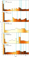
Fig. 3.. Discontinuous changes in the instantaneous reproduction number are accurately associated with NPI timings.

The detail of the early-stage dynamics for the scaled incidence, j_t, as in Fig. 2 and color-coded in each panel from light (1 individual/day) to dark (10³ individuals/day) tones, shows an underlying stepwise instantaneous reproduction number, R_t (black dots). The offset, Δ, between NPI timings (cyan vertical lines) and major R_t changes is indicated for each location in days as mean ± SD, with an overall offset for all locations of 0.22 ± 0.63 days.

Fig. 4.. The infection-to-death dynamics remains homogenous across locations and over time.

The time courses of R_t and j_t accurately track the major NPIs over a year with the same distribution of infection-to-death delay (average of 19.3 days and SD of 9.1 days). R_t, j_t, and NPI timings are represented as in Fig. 3. The offset, Δ, between NPI timings and major R_t changes are indicated for each location in days as mean ± SD, with an overall offset for all locations of −0.07 ± 0.92 days.

Fig. 5.. Super-resolution identification of NPI timings.

The distribution of the offset of NPI inferred times (orange bars, left axis), with 0.92 SD, is much narrower than the distribution of infection-to-death delay used in the inference process (gray curve, right axis), with 9.1 SD.

References

1. R. Szeliski, Computer Vision: Algorithms and Applications. (Springer-Verlag, ed. 2, 2022).
1. C. Payer, D. Štern, H. Bischof, M. Urschler, Regressing heatmaps for multiple landmark localization using CNNs, in Medical Image Computing and Computer-Assisted Intervention (2016), vol. 9901, pp. 230–238.
1. Li B., Ren W., Fu D., Tao D., Feng D., Zeng W., Wang Z., Benchmarking single-image dehazing and beyond. IEEE Trans. Image Process. 28, 492–505 (2019). - PubMed
1. von Diezmann L., Shechtman Y., Moerner W. E., Three-dimensional localization of single molecules for super-resolution imaging and single-particle tracking. Chem. Rev. 117, 7244–7275 (2017). - PMC - PubMed
1. Biemond J., Lagendijk R. L., Mersereau R. M., Iterative methods for image deblurring. Proc. IEEE 78, 856–883 (1990).