Mega-scale experimental analysis of protein folding stability in biology and design

Abstract

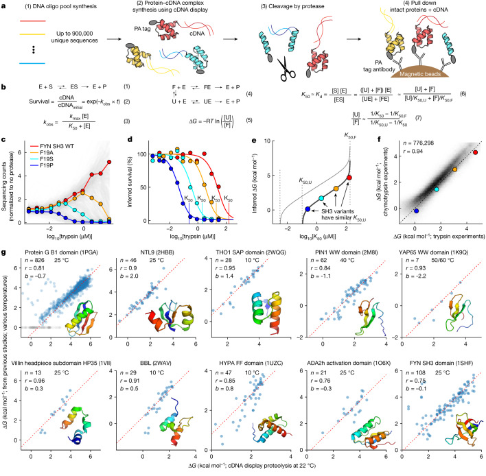
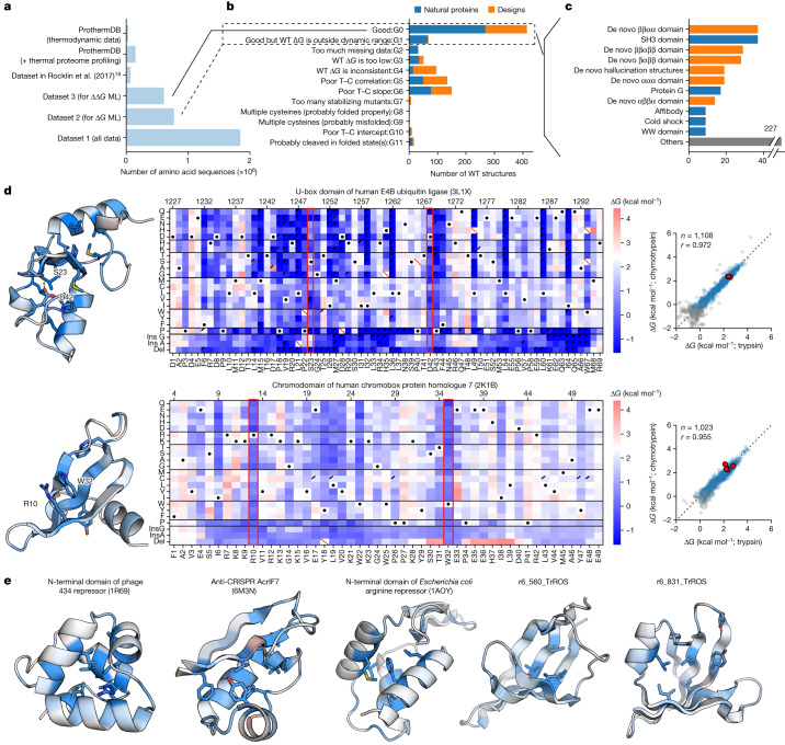
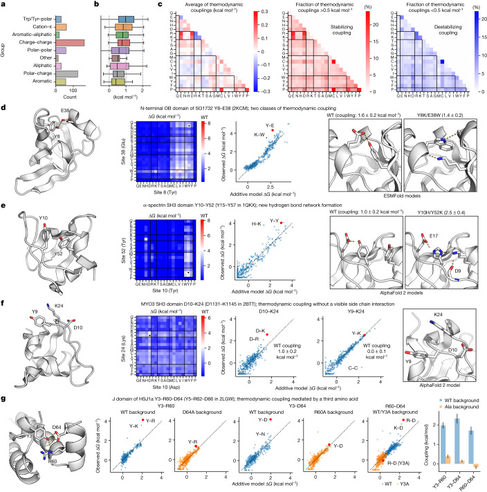
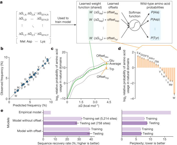
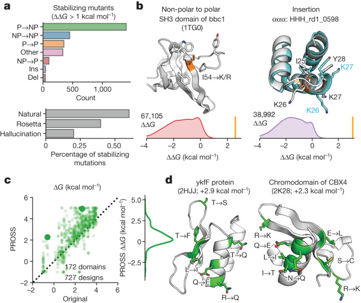
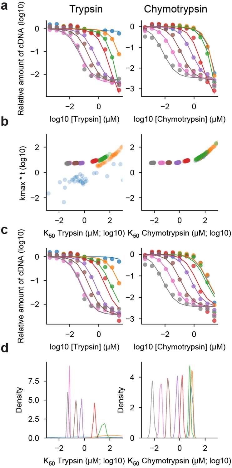
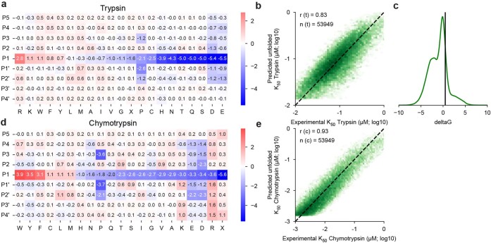
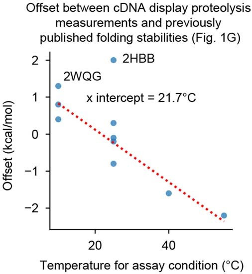
Advances in DNA sequencing and machine learning are providing insights into protein sequences and structures on an enormous scale¹. However, the energetics driving folding are invisible in these structures and remain largely unknown². The hidden thermodynamics of folding can drive disease^3,4, shape protein evolution^5-7 and guide protein engineering^8-10, and new approaches are needed to reveal these thermodynamics for every sequence and structure. Here we present cDNA display proteolysis, a method for measuring thermodynamic folding stability for up to 900,000 protein domains in a one-week experiment. From 1.8 million measurements in total, we curated a set of around 776,000 high-quality folding stabilities covering all single amino acid variants and selected double mutants of 331 natural and 148 de novo designed protein domains 40-72 amino acids in length. Using this extensive dataset, we quantified (1) environmental factors influencing amino acid fitness, (2) thermodynamic couplings (including unexpected interactions) between protein sites, and (3) the global divergence between evolutionary amino acid usage and protein folding stability. We also examined how our approach could identify stability determinants in designed proteins and evaluate design methods. The cDNA display proteolysis method is fast, accurate and uniquely scalable, and promises to reveal the quantitative rules for how amino acid sequences encode folding stability.

Fig. 1. cDNA display enables massively parallel measurement of protein folding stability.

a, A DNA oligonucleotide (oligo) library is expressed using cell-free cDNA display, producing proteins with an N-terminal 14-amino-acid PA tag and C-terminal covalent linkage to cDNA. After protease challenge, magnetic beads with anti-PA antibodies pull down proteins by their N termini. Sequencing the cDNA that is pulled down with the intact proteins enables quantification of the distribution of intact proteins. b, A thermodynamic model of proteolysis. (1) Protease enzymes (E) and protein substrates (S) form an ES complex to produce cleaved protein products (P). We model the cleavage as a first-order reaction (2) according to single-turnover kinetics (3). (4) Proteins are normally cleaved in the unfolded (U) state but can also be cleaved in the folded (F) state by cleaving the PA tag. We determine ΔG using each sequence’s measured K₅₀, a predicted sequence-specific K₅₀ for the unfolded state (K_50,U), and a universal K₅₀ for the folded state (K_50,F) (5–7). K_d, dissociation constant. k_obs, observed rate constant. c, Each human FYN SH3 variant sequence is shown as a grey line tracking its sequencing counts (fraction of the total library) relative to the pre-selection library. Four variants are highlighted in colour. WT, wild type. d, Inferred survival of uncleaved protein for four sequences from c at different protease concentrations (dots); lines show the global fit from the kinetic model. Vertical lines show inferred K₅₀ concentrations (one-half maximal cleavage rate, not 50% total cleavage). e, Relationship between K₅₀ and ΔG for different values of K_50,U. SH3 variants (coloured circles) all have similar K_50,U and fall on nearly the same ΔG versus K₅₀ line (black). Sequences with more cut sites have lower K_50,U and higher ΔG estimates for any K₅₀ (grey line). f, Consistency of ΔG estimates between independent trypsin and chymotrypsin experiments after quality filters (dataset 2), highlighting proteins shown in c. g, Our high-throughput ΔG measurements agree with published data from purified samples for mutants of the indicated domains (PDB IDs are in parentheses). Dashed lines show y = x + b (intercept). Grey points indicate missing reference data for the B1 domain of protein G. Plots indicate number of points (n), Pearson correlation (r), y-intercept (b) and the temperatures used for purified protein experiments (Supplementary Table 1). Insets show structural models.

Fig. 2. Comprehensive mutational analysis of stability in designed and natural proteins.

a, The size of existing datasets compared with our datasets 1, 2 and 3. Datasets 1, 2 and 3 are defined in Extended Data Table 1. ML, machine learning. b, Classification of mutational scanning results for each wild-type (WT) sequence. Each wild type sequence is included in only one group even when that wild-type meets multiple criteria (for example, both a poor slope and inconsistent intercept between trypsin and chymotrypsin (T–C)). c, Wild-type structures classified as G0 in b grouped into domain families. The 11 most common domain types are shown; additional classification shown in Supplementary Fig. 3. d, Mutational scanning results for the U-box domain of human E4B ubiquitin ligase (PDB ID: 3L1X) (top) and chromo domain of the chromobox protein homologue 7 (PDB ID: 2K1B) (bottom). Left, domain structures coloured by the average ΔΔG at each position; darker blue indicates that mutants are more destabilizing. Middle, heat maps show ΔG for substitutions, deletions and Gly and Ala insertions at each residue, with PDB numbering at top and our one-indexed numbering at bottom. White indicates wild-type stability, and red and blue indicate stabilizing and destabilizing mutations, respectively. Black dots indicate wild-type amino acids, red slashes indicate missing data and corner slashes indicate lower confidence ΔG estimates (95% confidence interval > 0.5 kcal mol⁻¹), including ΔG estimates near the edges of the dynamic range. Red boxes highlight the S23–D42 hydrogen bond in the U-box domain of human E4B ubiquitin ligase and the R10–W32 cation–π interaction in the chromo domain of the chromobox protein homologue 7. ΔG values were fitted to trypsin and chymotrypsin data together (Methods). Right, ΔG values independently determined using assays with trypsin (x axis) and chymotrypsin (y axis). Multiple codon variants of the wild-type sequence are shown in red, reliable ΔG values are in blue, and less reliable ΔG estimates are in grey. The black dashed line shows y = x. Plots show the number of reliable points and the Pearson r value for the blue (reliable) points. e, Structures of five other domains in our datasets, presented as in d. The two designed structures are AlphaFold models.

Fig. 3. Environmental factors that determine amino acid stabilities at a position.

a, Principal components (PC1–PC5) of the stability data showing the dominant trends for which amino acids are stabilizing or destabilizing at a site. We label each component with a biophysical interpretation and show the percentage of total variance explained by that component. Principal component analysis was performed using 20 features (ΔG with each amino acid variant) and 17,093 observations (sites in 365 domains). 325,132 ΔG measurements total. b, Relationships between the principal component values (x axis) for all 17,093 sites and environmental properties of those sites from the modelled 3D structure (y axis). Coloured lines show each environmental feature averaged over a window of 0.5 principal component units. Contacts indicate contact counts at those sites (Methods), counting all possible contacts (PC1 and PC5), only contacts to aromatic or aliphatic amino acids (PC3) or only contacts to acidic or basic amino acids (PC4). c, Structures of the C-terminal domain of NusG (PDB ID: 2MI6) with sites coloured by the value of PC1–PC5. Positive sites are stabilized by amino acids with positive loadings on that principal component (a). d, Mutational scanning results for NusG ordered by the value of PC1 at each site (not sequence order). The first five principal components at each site are shown at the top, coloured blue (negative) to pink (positive). The stability effects of each substitution are shown at the bottom, coloured blue (destabilizing) to red (stabilizing). Several positions with large (positive or negative) principal component values are highlighted to show the correspondence between principal component values and specific mutational stability patterns from c. e, Cumulative fraction of the total variance explained by the principal components, for separate principal component analyses of natural domains (blue), Rosetta designs (orange) and hallucination designs (green). Error bars show the s.d. from bootstrap resampling (n = 1,000) of the mutational scans but are too small to observe. f, Relationship between wild-type stability and variance (s.d.) in the ΔΔG data at each site, coloured as in e. Lines show LOWESS fits.

Fig. 4. Quantification of thermodynamic coupling between amino acid pairs.

a,b, Categorization of 559 pairs of amino acids in 190 domains selected for exhaustive double mutant analysis (210,000 ΔG measurements in total) (a) and thermodynamic couplings of wild-type amino acid pairs according to our additive model (b). In box plots, the centre line is the median, box limits delineate top and bottom quartiles and whiskers represent 1.5× the interquartile range (n = 559 in total). c, Average thermodynamic couplings (left) and fraction of pairs with positive (middle) or negative (right) couplings stronger than 0.5 kcal mol⁻¹ for all amino acid combinations (wild type and mutant). d,e, Thermodynamic coupling for N-terminal OB-domain of SO1732 (PDB ID: 2KCM) Y8–E38 (d) and α-spectrin SH3 domain (PDB ID: 1QKX) Y10–Y52 (Y15–Y57 in the PDB structure) (e). Left, domain structures showing the two mutated positions. Second from left, stabilities (ΔG) of all pairs at the two mutated positions. Second from right, agreement between stabilities from the additive model (x axis) and the observed stabilities (y axis, wild-type pair shown in red). Right, structural models of mutant pairs with strong couplings. Couplings show the observed stability minus the expected stability from the additive model; uncertainties show the s.d. from computing the couplings using 1,000 bootstrapped samples of the 400 double mutants. f, Thermodynamic coupling without a visible sidechain interaction in the MYO3 SH3 domain D10–K24 (D1131–K1145 in PDB ID 2BTT). Sub-panels as in d, with the magnified view of the wild-type structure of Y9, D10 and K24 shown on the right. g, Thermodynamic coupling mediated by a third amino acid in the J domain of HSJ1a: Y3–R60–D64 (Y5–R62–D66 in PDB ID 2LGW). Left, the AlphaFold-modelled structure of the HSJ1a J domain with three interacting amino acids. Scatter plots show the stabilities of double mutants in the additive model (x axis) and experimental data (y axis) in the wild-type background (blue) and with the third residue replaced by Ala (orange). Right, the thermodynamic coupling for each pair of wild-type amino acids in the wild-type (blue) and the Ala-substituted (orange) backgrounds (error bars represent the s.d. from bootstrap resampling (n = 1,000) as in d). Substituting any of the three amino acids for Ala eliminates the coupling between the other two.

Fig. 5. Amino acid frequencies in natural proteins systematically deviate from maximizing stability.

a, Classifier model for predicting wild-type amino acids from the folding stabilities (ΔG) of each protein variant. A shared weighting function converts the stabilities of protein variants with each amino acid into probabilities of those amino acids occurring (green). The probability for each amino acid is further modified by a constant amino acid-specific offset (orange). The model was parameterized using 99,156 ΔG measurements (5,214 sites in 90 non-redundant natural domains). b, Predicted and observed amino acid frequencies according to the classifier model after fitting. Amino acid frequencies were calculated for 5,214 sites. c, The weighting function from the classifier model after fitting (green). Grey lines show the weighting function after amino acid-specific offsets for Glu and Trp. In the region between 1.5 and 4 kcal mol⁻¹, the function has an approximately constant slope whereby a 1 kcal mol⁻¹ increase in stability leads to a 9.2-fold increase in amino acid probability (indicated by a dotted line). d, Relative offsets for 19 amino acids from the classifier model after fitting. Error bars show the s.d. of the model posterior (n = 25). At sites where ΔG_Val = ΔG_Trp, valine is around 11 times (=2⁰/2^−3.5) more likely to be the wild-type amino acid. e, The sequence recovery rate (left) and perplexity (right) for predicting wild-type amino acids using several models: a null model that ignores stability and always predicts amino acids at their observed frequencies, our classifier model without amino acid-specific offsets, and our full classifier model. Similar performance of the classifier model on a training set of 5,214 positions (light purple) and a testing set of 758 positions (dark purple) indicates that the model is not overfitted. Error bars show s.d. from bootstrap resampling (n = 1,000).

Fig. 6. Application of large-scale data to protein design.

a, Stabilizing mutations (ΔΔG > 1 kcal mol⁻¹) found in natural domains, Rosetta designs and hallucination designs, broken down by mutation type. NP, non-polar; P, polar; ins, insertion; del, deletion. Data are from 448,788 mutants in 412 domains. b, Two examples of stabilizing mutations found by our assay, along with the distribution of ΔΔG values for these mutation types. The highlighted mutations are indicated by vertical bars. Full mutational scanning results are shown in Supplementary Fig. 8. The structure of HHH_rd1_0598 is a design model reported previously, not an experimental structure. c, Stabilities of test domains before (x axis) and after (y axis) redesign by PROSS. The dashed black line represents y = x. Large dots indicate examples shown in d. Right, the distribution of ΔG change following PROSS redesign. Forty per cent of domains are stabilized by more than 1 kcal mol⁻¹ by the tool. d, AlphaFold models of domains redesigned by PROSS, with mutated amino acids in green. PDB ID and the change in stability are shown in brackets.

Extended Data Fig. 1. Single turnover model fitting on qPCR data.

(a) To test the single turnover model, we performed cDNA display proteolysis on a mixture of eight mini protein sequences with diverse folding stability and quantified the surviving amount of each cDNA using qPCR. We then each curve one at a time by Bayesian inference using the single turnover kinetics model in Fig. 1b. We sampled k_max*t and K₅₀ for each sequence. Dots represent the observed cDNA amount quantified by qPCR and lines show the two-parameter fits. (b) Posterior distributions of k_max*t and K₅₀ for eight proteins were shown. Whereas K₅₀ values vary between different proteins, k_max*t values (indicating saturation at high protease concentrations) were either constant or unconstrained by the data. (c) Based on the analysis (b), we fixed k_max*t at 10^0.65 and re-sampled K₅₀ for each protein. Dots represent the observed cDNA amount quantified by qPCR (same as in (a)) lines show the one-parameter fits. (d) Posterior distributions of K₅₀. For trypsin, the K₅₀ values for the two most stable proteins (orange and blue) could not be defined because they were too stable and outside of the dynamic range of this proteolysis assay.

Extended Data Fig. 2. Unfolded state model parameters and goodness of fit.

(a) Fit parameters for the unfolded state model position-specific scoring matrix (PSSM) for trypsin. The mean of all coefficients (−0.4) was subtracted from the values in the figure to aid visualization. Positive values indicate faster proteolysis and lower predicted K_50,U values. By using different prior distribution widths for different rows during fitting, we guided the strongest rate determinants into the center row of each matrix, which we label “P1” (the assay cannot actually identify the specific location of cutting). Overall, the heatmap resembles similar data as previously reported and is consistent with known trypsin specificity determinants, including the preference for R/K at P1, the inhibitory effect of P, and the unfavorability of D and E. (b) 2D-histogram showing the overall agreement between the trypsin model (predicted K_50,U, y-axis) and the data (experimental K₅₀, x-axis). Only scrambled sequences with inferred ΔG < 0.5 kcal/mol (where we can assume K₅₀ ≈ K_50,U) are shown (53,949 out of 64,238 total sequences used in training). The Pearson r value is shown. (c) Overall distribution of inferred ΔG of all scramble sequences. The vertical line represents 0.5 kcal/mol, which is a threshold used in (b). (d, e) As above, for chymotrypsin. As in our previous report, the coefficients resemble established features of chymotrypsin specificity, including the preference for F/Y/W followed by M/L at P1, the inhibitory effect of P at P3, P1’, and P2’, and the general unfavorability of D and E^–. The mean of all coefficients (−0.5) was subtracted from the values in the figure to aid visualization.

Extended Data Fig. 3. Relationship between offset in Fig. 1g and assay temperature.

Previous studies shown in Fig. 1g used diverse conditions including buffer, pH, ion strength, and temperature (see Supplementary Table 1)^,–. However, our measurements were all conducted in PBS at room temperature (approximately 22 °C). In general, the offsets observed in Fig. 1g are correlated to the temperatures used in the previous studies, suggesting that the assay temperature is the main cause of the offsets. The red line represents a best fit line. The x-intercept (21.7 °C) is close to our assay condition (approximately 22 °C). 2HBB (the N-terminal domain of Ribosomal Protein L9) and 2WQG (SAP domain from Tho1) were not included in the linear fit. 2HBB is an outlier; this may owe to its zinc-binding activity or to differences between the measured sequences (our construct lacks three C-terminal amino acids present in the previous study). 2WQG is close to the fit line but was removed because the previous literature used the L31W background as ‘wild-type’; this mutation stabilizes the protein by 0.49 kcal/mol.

Extended Data Fig. 4. Heat maps for a stable domain (Ubiquitin; 1UBQ) and its destabilizing mutants.

(a) Mutational scanning results for human erythrocytic ubiquitin (1UBQ) and its destabilizing mutant backgrounds (I3A and L67S). Heat maps show the ∆G of wild-type ubiquitin (top), ubiquitin I3A (middle-top), ubiquitin L67S (middle-bottom), and the difference (∆∆G) between two mutant backgrounds (bottom) for substitutions, deletions, and Gly and Ala insertions at each residue. In the three ∆G heat maps, white represents the folding stability of the wild-type and red/blue indicates stabilizing/destabilizing mutations. Black dots indicate the background (wild-type or mutant) amino acid, red slashes indicate missing data, and black corner slashes indicate lower confidence ∆G estimates, (95% confidence interval > 0.5 kcal/mol), including ∆G estimates near the edges of the dynamic range. (b) Consistency between mutant stabilities measured in the I3A background (x-axis) and L67S (y-axis) background. The plot is annotated with the number of points and the Pearson r value. (c) Ubiquitin structure highlighting the mutant points (I3 and L67) and the residues with a different effect on stability between two mutational backgrounds.

Extended Data Fig. 5. Consistency of K₅₀ measurements across libraries.

(a and b) To examine the consistency between K₅₀ (μM) values measured in different libraries, we included identical sequences (potentially with different padding at the termini) in multiple libraries. For each pair of libraries with overlapping sequences, we show the K₅₀ values for those sequences in both libraries for trypsin (a) and chymotrypsin (b). The top row shows raw K₅₀ values for overlapping sequences in each library; the second row shows the difference in K₅₀ estimates plotted against the K₅₀ in one of the libraries. The red diagonal line shows Y=X in the top row and Y = 0 (i.e. identical K₅₀ estimates) in the bottom row. Blue/orange vertical lines show K_50,F; all K₅₀ values above K_50,F are treated as equivalent. Each plot is annotated at the top-left with the total number of overlapping sequences and Pearson r-value between the libraries.

Extended Data Fig. 6. Domains with and without evidence of cleavage from the folded state.

(a) Mutational scanning results for 2L3X, which includes trypsin cleavage sites in the loop region. Left: Heat maps show the ∆G measurements from independent trypsin (top) and chymotrypsin challenges (bottom) for substitutions, deletions, and Gly and Ala insertions at each residue, with our one-indexed numbering at the bottom. Black dots indicate the wild-type amino acid, red slashes indicate missing data, and black corner slashes indicate lower confidence ∆G estimates, (95% confidence interval > 0.5 kcal/mol), including ∆G estimates near the edges of the dynamic range. The colored boxes highlight the flexible loop region. Right: Comparison of independent trypsin and chymotrypsin ∆G measurements. Multiple codon variants of the wild-type sequence are shown in red, reliable ∆G values in blue, and less reliable ∆G estimates (same as above) in gray. The black dashed line represents Y = X. The dots show a reverse ‘L’ shape because trypsin can cleave the loop even from the folded state, lowering the apparent stability for the wild-type and all high-stability variants. (b) 2L3X structure highlighting arginines in the loop region (R14 and R16). (c) Same as (a) for 2L3X after removing the trypsin-cleavable sites (R14 and R16) from the loop. In this deep mutational scanning, we observed higher consistency between trypsin and chymotrypsin challenges because we removed sites that could be cleaved in the folded state. (d) Top: Four example domains with long protease-cleavable loops that do not show evidence of folded state cleavage. Bottom: Agreement between mutant ∆G values independently determined using assays with trypsin (x-axis) and chymotrypsin (y-axis), as in (a). The consistency between the two proteases indicates that both proteases are measuring global unfolding, unlike the example in (a).

Extended Data Fig. 7. Comparison of ∆∆G observed in experiments and ∆∆G reconstructed by the PCs.

(a) Distribution of the mean ∆∆G values across all sites, using the experimental data (left) and ∆∆G values reconstructed from the principal components. More negative average ∆∆G values indicate greater stabilization from the wild-type amino acid. Center line, box limit, and whiskers represent median, upper and lower quartiles, and 1.5x interquartile range of each distribution (n = 17,093). (b) As in (a), grouped by domain types (natural domains, Rosetta designs, and hallucination designs). Center line, box limit, and whiskers represent median, upper and lower quartiles, and 1.5x interquartile range of each distribution (n = 17,093 in total).

Extended Data Fig. 8. Comparison of AlphaFold model and NMR structure for J domain of HSJ1a Structure of J domain in HSJ1a (2LGW).

We show NMR structure of all states stacked (a) and the first state (b), and AlphaFold predicted structures for the minimum construct (the variable segment in cDNA display) (c), the construct with linkers for cDNA display proteolysis (d), and the exact sequence used for NMR (e). In (f), we overlay the first state of the NMR ensemble (cyan) with the AlphaFold structure (orange) of the minimal construct.

Extended Data Fig. 9. Properties of functional sites across diverse domains.

(a) The relationship between wild-type stability (average ∆∆G for substitutions) and evolutionary-based sensitivity to substitutions (normalized averaged GEMME score). All sites above the orange dashed line are highly conserved but unimportant for stability; we define these as “functional sites”. (b) As in (a), highlighting positions in the HP1 chromo domain (2M2L; green) and the BBC1 SH3 domain (1TG0; red). (c) Structures of HP1 chromo domain and BBC1 SH3 domain (gray) and their ligands (light blue). Functional sites are shown in orange. Ligand positions were modeled based on PDB structures 1KNA (for HP1) and 2LCS (for the SH3 domain). (d) Amino acids are ranked by the percentage of positions where that wild-type amino acid is classified as functional, for positions in 104 non-redundant natural domains. (e) The percentage of functional residues in each of the 104 non-redundant domains. (f) Structures of the two domains with the highest percentages of functional residues. Nucleic acids interacting with each of the structures are shown in light blue and functional residues are shown in orange. The Sso7d-DNA complex is the crystal structure 1BNZ; the S19-RNA complex is modeled based on the 4V5Y structure. (g) As in (a), except only considering nonpolar substitutions for calculating ∆∆G and normalized averaged GEMME score. (h) The distributions of burial (side chain contacts) for all sites (blue), sites where the wild-type amino acid is unimportant for stability (average ∆∆G < 1 kcal/mol) (green), and functional sites (orange). Functional sites are generally located on the surface of the protein. Two unusual buried functional residues are highlighted. (i) Structure of the DUF1471 domain of yahO (2MA4) with functional sites in orange and the unusual buried functional site A64 in red. Ala64 is highly conserved yet the domain is stabilized by substitutions to Tyr or Phe (positive ∆∆G, x-axis). However, Tyr and Phe are rarely found in evolution (low GEMME score, y-axis). (j) Left: Structure of the N-terminal domain of FK506-binding protein 3 (2KFV) with functional sites in orange and the unusual buried functional site L55 (L78 in PDB numbering) in red. Middle: Residues with chemical shift perturbations in response to DNA binding; L55 shows a perturbation despite not contacting DNA. Right: L55 is conserved (high GEMME score, y-axis) but relatively unimportant for stability (low average ∆∆G, x-axis). Substitution to Phe, Val, or Ile is thermodynamically neutral (∆∆G near zero) but these amino acids are rarely found in evolution (low GEMME score).

Extended Data Fig. 10. Analysis of stable yet less hydrophobic designs and notable hydrogen bond networks.

(a) Relationship between hydrophobicity (calculated based on the previous report) and folding stability (∆G) for designed proteins. Examples from (b) are shown as large dots. (b) For three proteins with high folding stability and low hydrophobicity, we highlight critical hydrophilic interactions stabilizing these proteins. Gray density plots show the average ∆∆G of substitutions at 3,858 polar sites in 151 designed domains. Colored vertical bars show the values for the highlighted positions. These three proteins feature polar amino acids where the average ∆∆G of substitutions is unusually destabilizing (> top 5%ile). For HHH_rd1_0756, K22 is shown as a red line; the interacting W32 is considered nonpolar and not shown. Full mutational scanning results are shown in Supplementary Fig. 7. All three structures are design models reported previously, not experimental structures. (c) As in (a), highlighting EHEE_rd2_0152 (from (b)) and two other designs with the same hydrogen bond network. (d) Average ∆∆G of substitutions at 3,715 polar sites in 144 designed domains. The colored vertical bars indicate the values for the sites related to the 2nd hydrogen bond network shown in (b) for EHEE_rd2_0152. (e) Relationship between ∆∆G in EHEE_rd2_0152 and in the other designs EHEE_rd2_0372 or EHEE_rd2_0191 for E11, R14, and E18. At E11, substitutions to the 19 other amino acids have smaller effects in EHEE_rd2_0372 (blue) and EHEE_rd2_0191 (orange) compared to in EHEE_rd2_0152 (e.g. all points are above the dashed Y=X line). However, the points are ordered similarly; i.e. the rank ordering of the 19 other amino acid variants in stability is similar between the three designs. For R14 and E18, substitutions in EHEE_rd2_372 (blue) have similar effect sizes to EHEE_rd2_0152, but substitutions in EHEE_rd2_0191 (orange) have smaller effects. Again, the rank ordering of the amino acid variants by stability is similar across the three designs.

Extended Data Fig. 11. Global analysis of PROSS designs.

(a) All 727 PROSS designs grouped according to the number of amino acid substitutions in each design. Top: the number of designs with each different number of substitutions. Bottom: the distribution of design results for each group. ∆∆G indicates the stability of the PROSS design (∆G) minus the stability of the original wild-type sequence; positive ∆∆G indicates the design stabilized the domain. Center line, box limit, whiskers, and dots represent median, upper and lower quartiles, 1.5x interquartile range, and outliers of each distribution (n = 727 in total). (b) ∆∆G distributions for all amino acid substitutions in wild-type domains used as input to PROSS (blue), all amino acid substitutions at sites modified in PROSS designs (orange), and all PROSS-designed substitutions (green). All ∆∆G measurements are in the original wild-type background; positive ∆∆G indicates stabilizing substitutions. (c) Relationship between ∆∆G of PROSS designs and ∆∆G of the most stabilizing mutations designed by PROSS. At left, we compare PROSS designs to the single most stabilizing mutation (in the original wild-type background) out of all the substitutions in the PROSS design. At right, we compare PROSS designs to the sum of the two most stabilizing mutations (each measured individually in the original wild-type background without considering thermodynamic coupling). The density plots show the distribution of PROSS designs that were better (positive) or worse (negative) than the single best mutation (left) or sum of the two best mutations (right). Two-thirds of designs are better than the best single designed mutation, although the difference is small. Likewise, two-thirds of designs are worse than the additive effect of the two best designed mutations (assuming no thermodynamic coupling).

References

1. Jumper J, et al. Highly accurate protein structure prediction with AlphaFold. Nature. 2021;596:583–589. doi: 10.1038/s41586-021-03819-2. - DOI - PMC - PubMed
1. Dill KA. Dominant forces in protein folding. Biochemistry. 1990;29:7133–7155. doi: 10.1021/bi00483a001. - DOI - PubMed
1. Stein A, Fowler DM, Hartmann-Petersen R, Lindorff-Larsen K. Biophysical and mechanistic models for disease-causing protein variants. Trends Biochem. Sci. 2019;44:575–588. doi: 10.1016/j.tibs.2019.01.003. - DOI - PMC - PubMed
1. Yue P, Li Z, Moult J. Loss of protein structure stability as a major causative factor in monogenic disease. J. Mol. Biol. 2005;353:459–473. doi: 10.1016/j.jmb.2005.08.020. - DOI - PubMed
1. Agozzino L, Dill KA. Protein evolution speed depends on its stability and abundance and on chaperone concentrations. Proc. Natl. Acad. Sci. USA. 2018;115:9092–9097. doi: 10.1073/pnas.1810194115. - DOI - PMC - PubMed