Sequential Attractors in Combinatorial Threshold-Linear Networks

Abstract

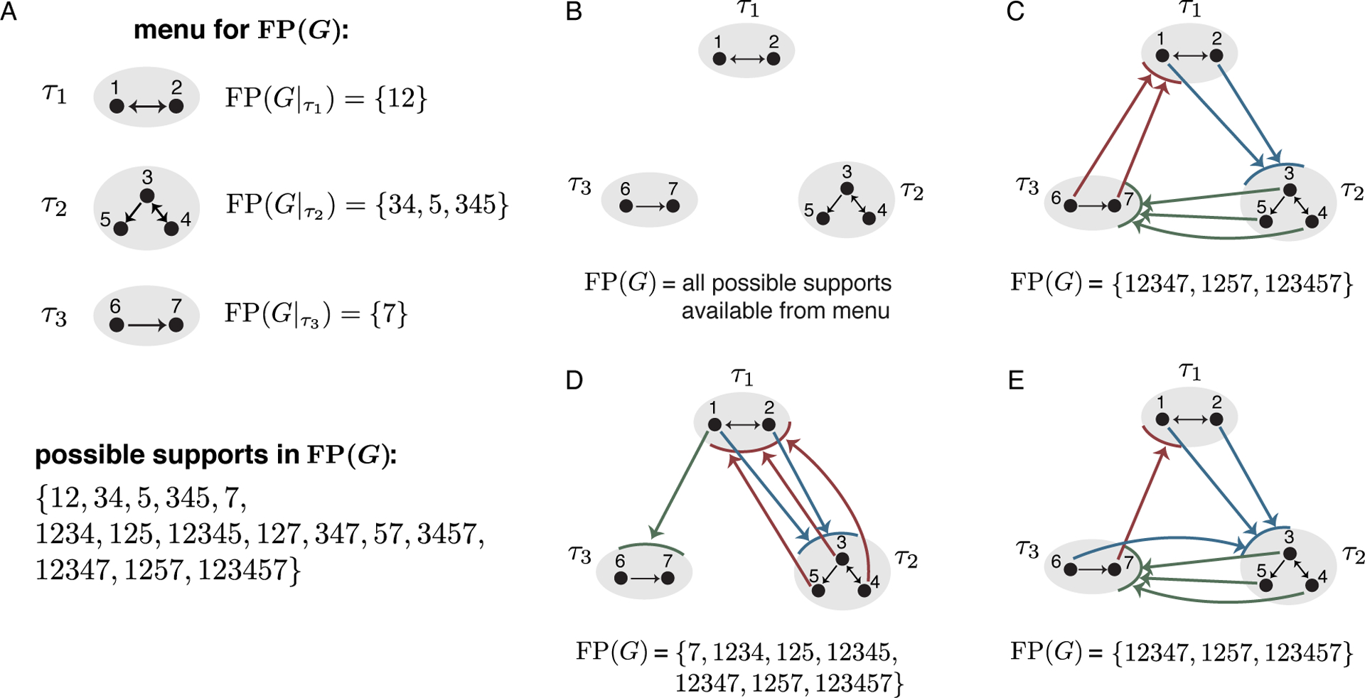
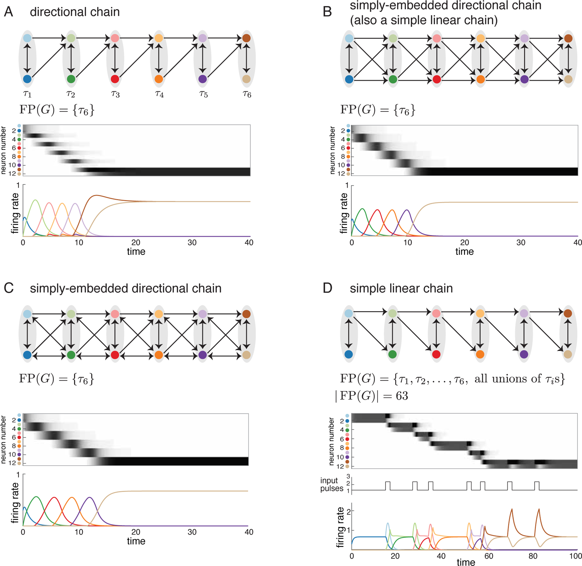
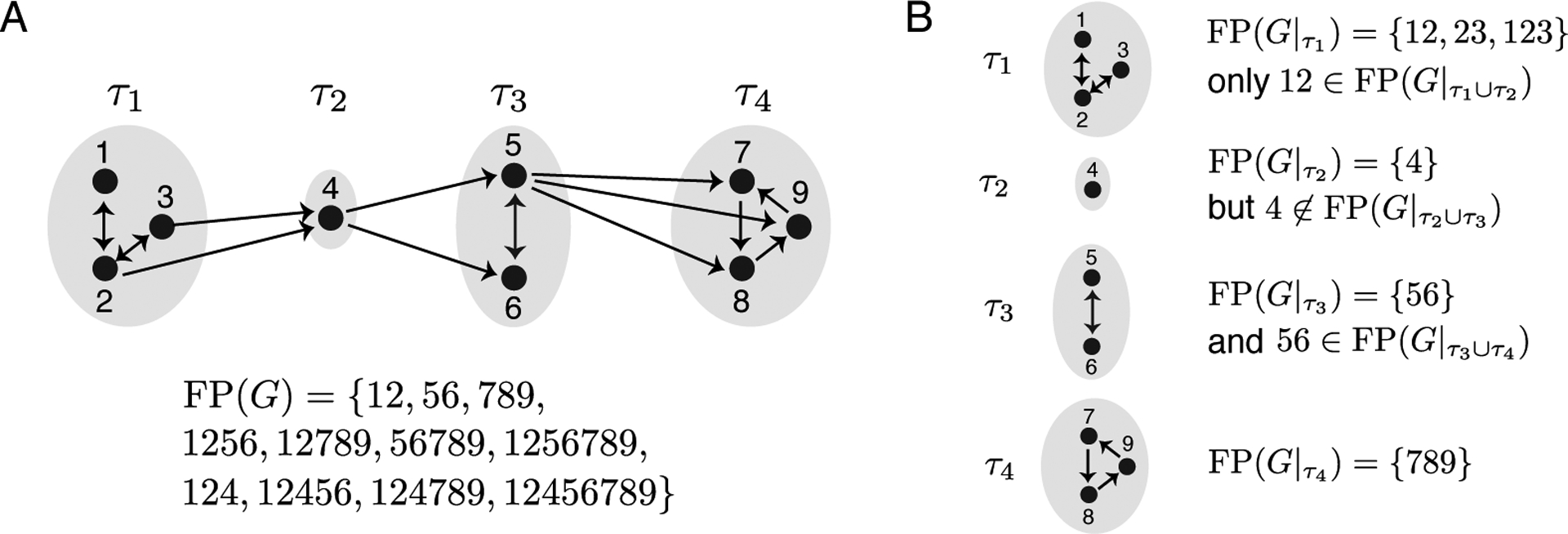
Sequences of neural activity arise in many brain areas, including cortex, hippocampus, and central pattern generator circuits that underlie rhythmic behaviors like locomotion. While network architectures supporting sequence generation vary considerably, a common feature is an abundance of inhibition. In this work, we focus on architectures that support sequential activity in recurrently connected networks with inhibition-dominated dynamics. Specifically, we study emergent sequences in a special family of threshold-linear networks, called combinatorial threshold-linear networks (CTLNs), whose connectivity matrices are defined from directed graphs. Such networks naturally give rise to an abundance of sequences whose dynamics are tightly connected to the underlying graph. We find that architectures based on generalizations of cycle graphs produce limit cycle attractors that can be activated to generate transient or persistent (repeating) sequences. Each architecture type gives rise to an infinite family of graphs that can be built from arbitrary component subgraphs. Moreover, we prove a number of graph rules for the corresponding CTLNs in each family. The graph rules allow us to strongly constrain, and in some cases fully determine, the fixed points of the network in terms of the fixed points of the component subnetworks. Finally, we also show how the structure of certain architectures gives insight into the sequential dynamics of the corresponding attractor.

Keywords: 34A34; 92C20; attractor dynamics; network architectures; neuronal sequences; threshold-linear networks.

Figure 1.

Sequential attractors from cycle graphs. (A)–(C) CTLNs corresponding to a 3-cycle, a 4-cycle, and a 5-cycle each produce a limit cycle where the neurons reach their peak activations in the expected sequence. Colored curves correspond to solutions $x_i\left(t\right)$ for matching node $i$ in the graph. (D) Attractors corresponding to the embedded 3-cycle, 4-cycle, and 5-cycle of the network are transiently activated to produce sequences matching those of the isolated cycle networks in (A)–(C). For each network in (A)–(D), $\mathrm{F}\mathrm{P}\left(G\right)$ is shown, with the minimal fixed points bolded. To simplify notation for $\mathrm{F}\mathrm{P}\left(G\right)$, we denote a subset $\left\{i_1,\dots ,i_k\right\}$ by $i_1\cdots i_k$. For example, 12345 denotes the set {1, 2, 3, 4, 5}. Unless otherwise noted (as in section 4), all simulations have CTLN parameters $\epsilon =0.25,\delta =0.5$, and $\theta =1$.

Figure 2.

Cyclic unions and related variations. (A) A cyclic union has component subgraphs with subsets of nodes ${\tau }_1,\dots ,{\tau }_N$, organized in a cyclic manner. While edges within each ${\left.G\right|}_{{\tau }_i}$ can be arbitrary, edges between components are determined as follows: every node in ${\tau }_i$ sends an edge to every node ${\tau }_{i+1}$, with ${\tau }_N$ sending edges to ${\tau }_1$. (B1), (C1), (D1) Three cyclic unions with firing rate plots showing solutions to a corresponding CTLN. Above each solution the associated sequence of firing rate peaks is given, with synchronously firing neurons denoted by parentheses. (B2), (C2), (D2) These graphs are all variations on the cyclic unions above them, with some edges added or dropped (highlighted in magenta). Solutions of the corresponding CLTNs qualitatively match the solutions of the corresponding cyclic unions. In each case, the sequence is identical.

Figure 3.

Example graphs generalizing cyclic union structure. (A) A cyclic union of component subgraphs ${\left.G\right|}_{{\tau }_1},\dots ,{\left.G\right|}_{{\tau }_3}$ together with its $\mathrm{F}\mathrm{P}\left(G\right)$ and the global attractor of its corresponding CTLN. (B)–(D) Different generalizations of the cyclic union structure of the graph in A. Each graph has the same component subgraphs ${\left.G\right|}_{{\tau }_1},\dots ,{\left.G\right|}_{{\tau }_3}$, but different conditions on the edges between these components. For each graph, $\mathrm{F}\mathrm{P}\left(G\right)$ and the global attractor are shown.

Figure 4.

Summary of main results. In each graph, colored edges from a node to a component indicate that the node projects edges out to all the nodes in the receiving component, as needed for a simply-embedded partition. Thick gray edges indicate directionality of the subgraph ${\left.G\right|}_{{\tau }_i\cup {\tau }_{i+1}}$.

Figure 5.

Cyclic union, simply-embedded directional cycle, their dynamics and $\mathbf{F}\mathbf{P}\left(\mathit{G}\right)$. (A) (Top) A cyclic union $G_1$ with component subgraphs ${\left.G\right|}_{{\tau }_1},\dots ,{\left.G\right|}_{{\tau }_4}$. Thick colored edges from a node to a component indicate that the node projects edges out to all the nodes in the receiving component. (Bottom) A solution for the corresponding CTLN. (B) (Top) A simply-embedded directional cycle $G_2$ with the same component subgraphs as $G_1$. (Bottom) A solution for the corresponding CTLN with the same initial condition as the network in panel A. The solution of this network is qualitatively the same as that for the network in A except that the period is twice as long (note the different time axes). (C) (Left) The fixed point supports $\mathrm{F}\mathrm{P}\left({\left.G\right|}_{{\tau }_i}\right)$ of each component subgraph. (Right) $\mathrm{F}\mathrm{P}\left(G\right)$ is identical for both $G_1$ and $G_2$: it consists of unions of component fixed point supports, exactly one per component. To highlight this structure of all the fixed point supports, the portion of each support that each ${\tau }_i$ is color-coded.

Figure 6.

Uniform in-degree graphs. (A) All $n=3$ graphs with uniform in-degree. (B) Cartoon showing survival rule for an arbitrary subgraph with uniform in-degree d.

Figure 7.

The three cases of graphical domination in Rule 2. In each panel, $k$ graphically dominates $j$ with respect to $\sigma$ (the outermost shaded region). The inner shaded regions illustrate the subsets of nodes that send edges to $j$ and $k$. Note that the vertices sending edges to $j$ are a subset of those sending edges to $k$, but this containment need not be strict. Dashed arrows indicate optional edges between $j$ and $k$.

Figure 8.

Directional graphs: examples and non-examples. (A) Example directional graphs and their $\mathrm{F}\mathrm{P}\left(G\right)$. On the right, solutions for A3 and A6 are shown where the activity was initialized on the nodes in $\omega$. (B) Example nondirectional graphs with their $\mathrm{F}\mathrm{P}\left(G\right)$, as well as solutions for the networks in B2 and B3.

Figure 9.

Family of directional graphs.

Figure 10.

Pairwise chaining of two directional graphs. (Left) Two directional graphs $G_1$ and $G_2$ with direction ${\omega }_i\to {\tau }_i$, where ${\left.G_1\right|}_{{\tau }_1}={\left.G_2\right|}_{{\omega }_2}$. (Right) The graph $G_1\bigsqcup G_2$ formed from chaining together $G_1$ and $G_2$ by identifying ${\tau }_1$ with ${\omega }_2$. By Lemma 2.6, $G_1\bigsqcup G_2$ is directional for $\omega ={\omega }_1\cup {\omega }_2$ (in gray) and $\tau ={\tau }_2$ (in green).

Figure 11.

Directional chain. A cartoon of a directional chain with components ${\tau }_0,{\tau }_1,\dots ,{\tau }_N$. For each $i=1,\dots ,N$, the induced subgraph ${\left.G_i\stackrel{\text{def}}{=}G\right|}_{{\tau }_{i-1}\cup {\tau }_i}$ is directional. The arrows between components indicate the directionality ${\tau }_{i-1}\to {\tau }_i$. Note there may be edges in both directions between adjacent components, as in the example directional graphs in Figure 8, but there are no edges between nonadjacent components.

Figure 12.

Directional chain and directional cycle. (A) A graph built from chaining together directional graphs $G_1,\dots ,G_4$, where $G_i={\left.G\right|}_{{\tau }_{i-1}\cup {\tau }_i}$. (B) A solution of the CTLN for the directional chain in A when the activity is initialized on nodes 1 and 2. Activity flows through the chain, eventually stabilizing on the fixed point attractor of ${\tau }_4$. (C) A solution of the CTLN for the directional cycle obtained from the graph in A by identifying ${\tau }_4$ with ${\tau }_0$ to make the chain wrap cyclically wrap around. The activity is initialized on nodes 1 and 2 and falls into a limit cycle hitting all the components ${\tau }_i$ in cyclic order.

Figure 13.

Illustrations for Theorem 1.2 and Lemma 2.10. (A) A cartoon of a directional cycle; each pastel colored blob is a directional graph $G_i$ with direction ${\omega }_i={\tau }_{i-1}\to {\tau }_i$ indicated by arrows along the outside. Note that all vertices of $G$ lie within an overlap of adjacent $G_i$, but each $G_i$ has edges between the two overlaps ${\tau }_{i-1}$ and ${\tau }_i$. Within the directional cycle, a fixed point support $\sigma \in \mathrm{F}\mathrm{P}\left(G\right)$ is shown in dark gray. Theorem 1.2 guarantees that ${\left.G\right|}_{\sigma }$ contains an undirected cycle that hits all the ${\tau }_i$ in cyclic order (shown in magenta). The vertices in the cycle are labeled following the notation for the proof of Theorem 1.2. (B) Cartoon for setup of Lemma 2.10. The pale pink and blue blobs depict overlapping directional graphs $G_{i-1}$ and $G_i$. The restriction of fixed point support $\sigma \in FP\left(G\right)$ to this subgraph is shown with its component subgraphs ${\sigma }_i\stackrel{\text{def}}{=}\sigma \cap \left({\omega }_i\cup {\tau }_i\right)$ denoted with light gray blobs. The subgraph ${\left.G\right|}_{{\sigma }_i}$ can be broken into its connected components, and ${\alpha }_i$ (dark gray) denotes one such component. There exists a $j\in {\alpha }_i\cap {\omega }_i$ such that $j$ is dominated by some $k$ in $G_i$ with respect to ${\alpha }_i$. Then Lemma 2.10 guarantees that there is some $\ell \in {\sigma }_{i-1}\cap {\omega }_{i-1}$ such that $\ell \to j$.

Figure 14.

Graphs with a simply-embedded partition from Example 3.1. (A) (Top) A collection of component subgraphs with their $\mathrm{F}\mathrm{P}\left({\left.G\right|}_{{\tau }_i}\right)$. (Bottom) The set of possible fixed point supports for any graph that has these subgraphs in the simply-embedded partition. (B)–(E) Example graphs with a simply-embedded partition with the component subgraphs from A, together with their $\mathrm{F}\mathrm{P}\left(G\right)$. In (C)–(E), thick colored edges from a node to a component indicate that the node projects edges out to all the nodes in the receiving component.

Figure 15.

Graph with two nontrivial simply-embedded partitions. The panels show two drawings of the same graph $G$ to highlight two partitions: (A) the simply-embedded partition {1 |2, 3, 4| 5}, (B) the Simply-embedded partition {2 |1, 3, 5| 4}.

Figure 16.

Directional chains versus simple linear chains. (A)–(C) Graphs that are directional chains. Activity initialized on ${\tau }_1$ flows through the chain, hitting each component in sequence, and converging on the nodes of ${\tau }_6$. (D) A simple linear chain that is not directional. Each component clique supports a stable fixed point of the network. Unions of these component fixed point supports also yield fixed points. Activity initialized on ${\tau }_1$ would stay indefinitely at the corresponding stable fixed point. Small kicks to the $\theta$ input (labeled as input pulses on the plot) can cause the activity to fall out of the current stable fixed point and move forward to converge onto ${\tau }_{i+1}$. At time 60, the activity has converged to ${\tau }_6$. After this point, all additional input pulses lead to increases in the activity of the nodes in ${\tau }_6$, but the activity can never escape the final stable fixed point of the chain.

Figure 17.

Simple linear chain. (A) An example simple linear chain together with its $\mathrm{F}\mathrm{P}\left(G\right)$. The first row of $\mathrm{F}\mathrm{P}\left(G\right)$ gives the surviving fixed points from each component subgraph; the second row shows that all unions of these component fixed points are also in $\mathrm{F}\mathrm{P}\left(G\right)$ (Theorem 3.6(ii)); the third row shows the additional fixed point supports in $\mathrm{F}\mathrm{P}\left(G\right)$ that arise from the broader menu (Theorem 3.6(i)). (B) $\mathrm{F}\mathrm{P}\left({\left.G\right|}_{{\tau }_i}\right)$ for each component subgraph from A, and the list of which of these supports survive the addition of the next component in the chain.

Figure 18.

Simple feedforward network. A feedforward network generalizing the conditions of the simple linear chain. Notice that $\mathrm{F}\mathrm{P}\left(G\right)$ is not closed under unions of surviving component fixed points, since $\mathrm{123,456}\in FP\left(G\right)$ but $123456\notin FP\left(G\right)$.

Figure 19.

Strongly simply-embedded partitions. Four example graphs with a strongly simply-embedded partition, characterized by the fact that each node treats all the other components identically. Thus, any node that sends an edge out to one component must in fact send edges out to every component (i.e., it must be a projector onto the rest of the graph). Projector nodes are colored brown. (A) A disjoint union. (B) A clique union. (C)–(D) Example graphs with a mix of projector and nonprojector nodes within each component.

Figure 20.

Strongly simply-embedded partition with $\mathrm{F}\mathrm{P}\left(G\right)$. (A) A graph with a strongly simply-embedded partition $\left\{{\tau }_1\left|{\tau }_2\right|{\tau }_3\right\}$. Projector nodes are colored brown. (B) (Top) $\mathrm{F}\mathrm{P}\left({\left.G\right|}_{{\tau }_i}\right)$ for each component subgraph together with the supports from each component that survive within the full graph. (Bottom) $\mathrm{F}\mathrm{P}\left(G\right)$ for the strongly simply-embedded partition graph. The first two lines of $\mathrm{F}\mathrm{P}\left(G\right)$ consist of unions of surviving fixed points, at most one per component. The third line gives the fixed points that are unions of dying fixed point supports, exactly one from every component.

Figure 21.

Example graphs of size 5. A collection of example $n=5$ graphs of different types and their corresponding dynamic attractors for $\epsilon =0.51,\delta =1.76,\theta =1$. The graphs are numbered following the ordering given in [9], which extensively catalogued $\mathrm{F}\mathrm{P}\left(G\right)$ and the dynamic attractors for all graphs of size 5 for this parameter choice.

Figure 22.

The three directional cycle representations of graph 21. (A) The simply-embedded directional cycle representation of graph 21. (B)–(C) Directional cycle representations that are not from a simply-embedded partition. (D) The global attractor of the CTLN for graph 21 with $\epsilon =0.51,\delta =1.76,\theta =1$. The sequence of neural firing matches that of both of the directional cycle representations from A and B. But the structure of the attractor (with neurons 1 and 5 high firing) is best represented by the simply-embedded directional cycle from A, since singleton components yield the high-firing neurons in directional cycles.

References

1. Abeles M, Local Cortical Circuits: An Electrophysiological Study, Springer, Berlin, 1982.
1. Arriaga M and Han EB, Dedicated hippocampal inhibitory networks for locomotion and immobility, J. Neurosci, 37 (2017), pp. 9222–9238. - PMC - PubMed
1. Aviel Y, Pavlov E, Abeles M, and Horn D, Synfire chain in a balanced network, Neurocomput., 44 (2002), pp. 285–292.
1. Bel A, Cobiaga R, Reartes W, and Rotstein HG, Periodic solutions in threshold-linear networks and their entrainment, SIAM J. Appl. Dyn. Syst, 20 (2021), pp. 1177–1208.
1. Biswas T and Fitzgerald JE, A Geometric Framework to Predict Structure from Function in Neural networks, https://arxiv.org/abs/2010.09660, 2022. - PMC - PubMed
LinkOut - more resources