AI Body Composition in Lung Cancer Screening: Added Value Beyond Lung Cancer Detection

Abstract

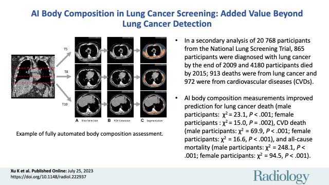
Background An artificial intelligence (AI) algorithm has been developed for fully automated body composition assessment of lung cancer screening noncontrast low-dose CT of the chest (LDCT) scans, but the utility of these measurements in disease risk prediction models has not been assessed. Purpose To evaluate the added value of CT-based AI-derived body composition measurements in risk prediction of lung cancer incidence, lung cancer death, cardiovascular disease (CVD) death, and all-cause mortality in the National Lung Screening Trial (NLST). Materials and Methods In this secondary analysis of the NLST, body composition measurements, including area and attenuation attributes of skeletal muscle and subcutaneous adipose tissue, were derived from baseline LDCT examinations by using a previously developed AI algorithm. The added value of these measurements was assessed with sex- and cause-specific Cox proportional hazards models with and without the AI-derived body composition measurements for predicting lung cancer incidence, lung cancer death, CVD death, and all-cause mortality. Models were adjusted for confounding variables including age; body mass index; quantitative emphysema; coronary artery calcification; history of diabetes, heart disease, hypertension, and stroke; and other PLCO_M2012 lung cancer risk factors. Goodness-of-fit improvements were assessed with the likelihood ratio test. Results Among 20 768 included participants (median age, 61 years [IQR, 57-65 years]; 12 317 men), 865 were diagnosed with lung cancer and 4180 died during follow-up. Including the AI-derived body composition measurements improved risk prediction for lung cancer death (male participants: χ² = 23.09, P < .001; female participants: χ² = 15.04, P = .002), CVD death (males: χ² = 69.94, P < .001; females: χ² = 16.60, P < .001), and all-cause mortality (males: χ² = 248.13, P < .001; females: χ² = 94.54, P < .001), but not for lung cancer incidence (male participants: χ² = 2.53, P = .11; female participants: χ² = 1.73, P = .19). Conclusion The body composition measurements automatically derived from baseline low-dose CT examinations added predictive value for lung cancer death, CVD death, and all-cause death, but not for lung cancer incidence in the NLST. Clinical trial registration no. NCT00047385 © RSNA, 2023 Supplemental material is available for this article. See also the editorial by Fintelmann in this issue.

Graphical abstract

Figure 1:

Example of fully automated body composition assessment in the lung cancer screening noncontrast low-dose chest CT scan in a 57-year-old male participant. (A) CT axial plane levels corresponding to the fifth (T5), eighth (T8), and 10th (T10) vertebral bodies were predicted. Corresponding axial CT sections were selected for body composition assessment. (B) The field of view (FOV) of each CT section with body section truncation was extended with missing body section imputation. (C) Areas of subcutaneous adipose tissue (SAT) (blue) and skeletal muscle (SM) (orange) were segmented on the field-of-view extended sections. Body composition measurements include SM index (166.2, normal group), SM attenuation (17.5 HU, lower group), SM SD (41.0 HU, normal group), SAT index (189.7, higher group), SAT attenuation (−88.4 HU, normal group), and SAT SD (28.0 HU, higher group). Indexes were calculated as summed area (in square centimeters) across three levels divided by participant height squared (in square meters).

Figure 2:

Cohort selection flowchart. A total of 2963 participants were excluded from body composition analysis due to missing baseline CT data (n = 312), image data corruption (n = 81), images failing the section thickness or scan length requirement (n = 158), or images failing the requirement for soft-tissue reconstruction kernels (n = 2412). Then, 1408 participants were excluded due to images failing the quality review process (n = 233) or to missing clinical data or end point ascertainment (n = 1175). DICOM = Digital Imaging and Communications in Medicine, NIfTI = Neuroimaging Informatics Technology Initiative.

Figure 3:

Pairwise associations of subcutaneous adipose tissue (SAT) index with SAT attenuation, skeletal muscle (SM) index, and SM attenuation of participants included in statistical analysis (20 768 participants: 12 317 male and 8451 female). Spearman correlation coefficients (ρ) were used to quantitatively assess the associations for male, female, and all participants separately. (A) Scatterplot shows the association between SAT index and SM index. Analysis indicated weak (0.20 ≤ |ρ| < 0.40) positive correlations between SAT index and SM index in male (ρ = 0.28) and female participants (ρ = 0.38) and a very weak (|ρ| < 0.20) negative correlation when combined (ρ = −0.10). Separation in the joint distributions of male and female participants was observed, with male participants showing a higher SM index and a lower SAT index, while female participants showed a lower SM index and a higher SAT index. (B) Scatterplot shows the association between SAT index and SAT attenuation. Strong (|ρ| ≥ 0.60) negative correlations were observed between SAT index and SAT attenuation in male (ρ = −0.68), female (ρ = −0.61), and all (ρ = −0.75) participants. Nonlinear correlation patterns can be observed in the joint distributions approximated by the scatterplot. (C) Scatterplot shows the association between SAT index and SM attenuation. Analysis indicated moderate (0.40 ≤ |ρ| < 0.60) negative correlations between SAT index and SM attenuation in male (ρ = −0.55) and female participants (ρ = −0.56) and a strong negative correlation when combined (ρ = −0.62).

Figure 4:

Estimated cumulative incidence functions of each end point in male participants (n = 12 317) stratified by skeletal muscle (SM) attenuation values of 27.6 HU (25th percentile) and 35.1 HU (75th percentile) as lower (<27.6 HU), normal (between 27.6 HU and 35.1 HU), and higher (>35.1 HU) groups. Solid step lines represent estimated cumulative incidence functions, while semitransparent bands represent 95% CIs. P values were derived with use of the Gray test for separation between cumulative incidence functions. (A) Plot displays the estimated cumulative incidence of lung cancer for each group. Compared with the normal group, the lower group exhibited a higher incidence of lung cancer, while the higher group exhibited a lower incidence of lung cancer. (B) Plot displays the estimated cumulative incidence of lung cancer death for each group. Compared with the normal group, the lower group exhibited a higher incidence of lung cancer death, while the higher group exhibited a lower incidence of lung cancer death. (C) Plot displays the estimated cumulative incidence of cardiovascular disease (CVD) death for each group. Compared with the normal group, the lower group exhibited a higher incidence of CVD death, while the higher group exhibited a lower incidence of CVD death. (D) Plot displays the estimated cumulative incidence of all-cause death for each group. Compared with the normal group, the lower group exhibited a higher incidence of all-cause death, while the higher group exhibited a lower incidence of all-cause death.

Figure 5:

Estimated cumulative incidence functions of each end point in female participants (n = 8451) stratified by skeletal muscle (SM attenuation) values of 23.0 HU (25th percentile) and 30.6 HU (75th percentile) as lower (<23.0 HU), normal (between 23.0 HU and 30.6 HU), and higher (>30.6 HU) groups. Solid step lines represent estimated cumulative incidence functions, while semitransparent bands represent 95% CIs. P values were derived with use of the Gray test for separation between cumulative incidence functions. (A) Plot displays the estimated cumulative incidence of lung cancer for each group. Separation of cumulative incidence functions was not observed (P = .11). (B) Plot displays the estimated cumulative incidence of lung cancer death for each group. Compared with the lower and normal groups, the higher group exhibited a lower incidence of lung cancer death. (C) Plot displays the estimated cumulative incidence of cardiovascular disease (CVD) death for each group. Compared with the normal group, the lower group exhibited a higher incidence of CVD death, while the higher group exhibited a lower incidence of CVD death. (D) Plot displays the estimated cumulative incidence of all-cause death for each group. Compared with the normal group, the lower group exhibited a higher incidence of all-cause death, while the higher group exhibited a lower incidence of all-cause death.

Figure 6:

Estimated unadjusted hazard ratios (HRs) of the lower and higher groups, with the normal group as reference for each body composition measurement (rows) and each end point event (columns) in male and female participants. The groups were obtained by the stratification based on the sex-specific 25th and 75th percentiles for each measurement. (A) Plot displays the estimated unadjusted HRs in male participants (n = 12 317). (B) Plot displays the estimated unadjusted HRs in female participants (n = 8451). The dots represent the estimated HRs. The segments represent the 95% CIs of the estimated HRs. The HR of 1 (no difference in hazard) is displayed as a red line in each plot for reference. The numbers following each dot-segment combination show the numerical value of the HR, with the 95% CI in parentheses and the associated P value in square brackets. For instance, as indicated by the fourth row in the column “CVD Death (n = 680)” in A, the lower skeletal muscle (SM) attenuation group in male participants (<27.6 HU) was associated with higher risk for cardiovascular disease (CVD) death (HR, 2.27 [95% CI: 1.93, 2.67]; P < .001) when compared with the normal group, which is consistent with observations in Figure 4C based on cumulative incidence functions. SAT = subcutaneous adipose tissue.

References

1. Heshka S , Ruggiero A , Bray GA , et al. Altered body composition in type 2 diabetes mellitus . Int J Obes 2008. ; 32 ( 5 ): 780 – 787 . - PMC - PubMed
1. Dulloo AG , Jacquet J , Solinas G , Montani JP , Schutz Y . Body composition phenotypes in pathways to obesity and the metabolic syndrome . Int J Obes 2010. ; 34 ( Suppl 2 ): S4 – S17 . - PubMed
1. Eid AA , Ionescu AA , Nixon LS , et al. Inflammatory response and body composition in chronic obstructive pulmonary disease . Am J Respir Crit Care Med 2001. ; 164 ( 8 Pt 1 ): 1414 - 1418 . - PubMed
1. Goodpaster BH , Park SW , Harris TB , et al. The loss of skeletal muscle strength, mass, and quality in older adults: the health, aging and body composition study . J Gerontol A Biol Sci Med Sci 2006. ; 61 ( 10 ): 1059 – 1064 . - PubMed
1. Troschel AS , Troschel FM , Best TD , et al. Computed tomography-based body composition analysis and its role in lung cancer care . J Thorac Imaging 2020. ; 35 ( 2 ): 91 – 100 . - PubMed
Publication types
Associated data