

Concept for the Real-Time Monitoring of Molecular Configurations during Manipulation with a Scanning Probe Microscope
- PMID: 37492192
- PMCID: PMC10364088
- DOI: 10.1021/acs.jpcc.3c02072
Concept for the Real-Time Monitoring of Molecular Configurations during Manipulation with a Scanning Probe Microscope
Abstract
A bold vision in nanofabrication is the assembly of functional molecular structures using a scanning probe microscope (SPM). This approach requires continuous monitoring of the molecular configuration during manipulation. Until now, this has been impossible because the SPM tip cannot simultaneously act as an actuator and an imaging probe. Here, we implement configuration monitoring using experimental data other than images collected during the manipulation process. We model the manipulation as a partially observable Markov decision process (POMDP) and approximate the actual configuration in real time using a particle filter. To achieve this, the models underlying the POMDP are precomputed and organized in the form of a finite-state automaton, allowing the use of complex atomistic simulations. We exemplify the configuration monitoring process and reveal structural motifs behind measured force gradients. The proposed methodology marks an important step toward the piece-by-piece creation of supramolecular structures in a robotic and possibly automated manner.
© 2023 The Authors. Published by American Chemical Society.
Conflict of interest statement
The authors declare no competing financial interest.
Figures
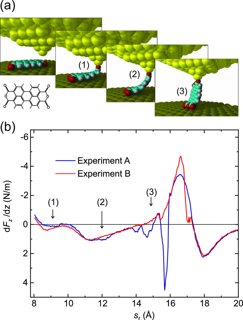
 , which contains all 47 stable molecular
configurations resulting from our molecular mechanics state transition
model for a given exemplary SPM tip position at sz = 10 Å. The primary degree of
freedom is the azimuthal angle of the molecule.
, which contains all 47 stable molecular
configurations resulting from our molecular mechanics state transition
model for a given exemplary SPM tip position at sz = 10 Å. The primary degree of
freedom is the azimuthal angle of the molecule.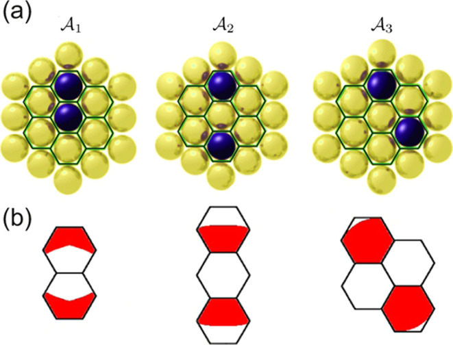
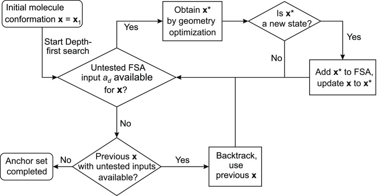
 . Once the depth-first search is complete,
the algorithm will repeat with a new initial state x1 from the next anchor set.
. Once the depth-first search is complete,
the algorithm will repeat with a new initial state x1 from the next anchor set.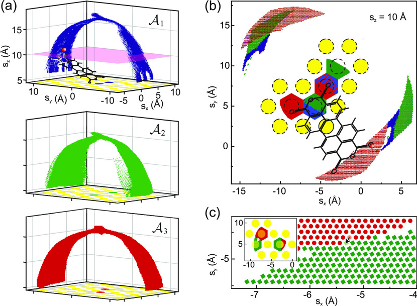
 . The lateral positions of Au atoms are
displayed in yellow, with the anchor atoms in the corresponding color.
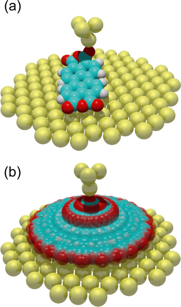
As exemplified in the upper panel, each point in the displayed cloud
of tip positions stands for a full configuration x of
the tip–molecule–surface junction. (b) Horizontal cut
through the s cloud of the three anchor sets at sz = 10 Å (the pink plane in panel (a)).
Au atoms are shown in yellow, and the reachable positions of the two
bottom Ocarb atoms (see Figure 4) are shown in the color of the respective
anchor set. An exemplary molecule in
. The lateral positions of Au atoms are
displayed in yellow, with the anchor atoms in the corresponding color.
As exemplified in the upper panel, each point in the displayed cloud
of tip positions stands for a full configuration x of
the tip–molecule–surface junction. (b) Horizontal cut
through the s cloud of the three anchor sets at sz = 10 Å (the pink plane in panel (a)).
Au atoms are shown in yellow, and the reachable positions of the two
bottom Ocarb atoms (see Figure 4) are shown in the color of the respective
anchor set. An exemplary molecule in  is drawn in black, with a red sphere marking
the corresponding tip position. (c) A tip displacement step (black
arrow) causes one anchor atom to change (white arrow in the inset,
length exaggerated for better visibility), such that the molecule
configuration moves from
is drawn in black, with a red sphere marking
the corresponding tip position. (c) A tip displacement step (black
arrow) causes one anchor atom to change (white arrow in the inset,
length exaggerated for better visibility), such that the molecule
configuration moves from  to
to  . Note that in panel (c), duplicate anchor
sets are displayed, which are rotated and translated with respect
to the primary anchor sets shown in panels (a) and (b).
. Note that in panel (c), duplicate anchor
sets are displayed, which are rotated and translated with respect
to the primary anchor sets shown in panels (a) and (b).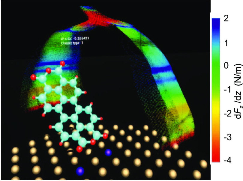
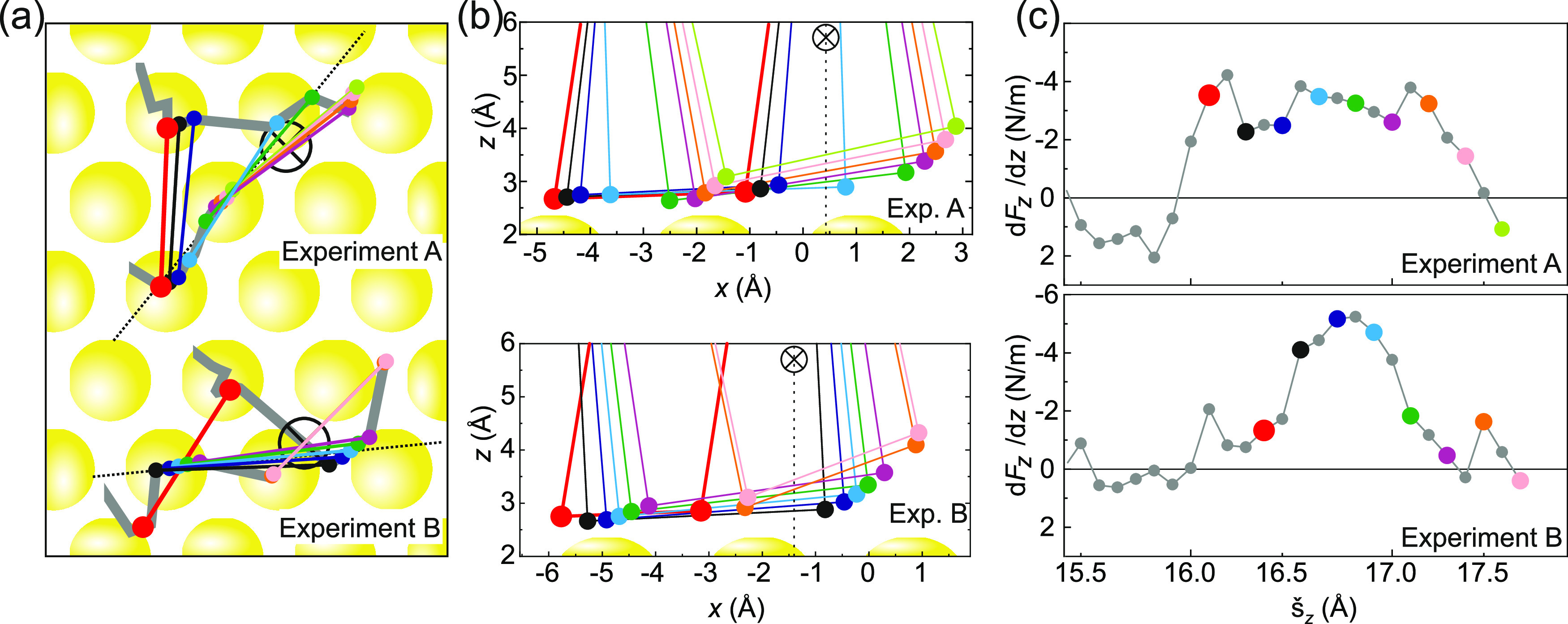
 ) is represented by a dot, the color of
which encodes the force gradient in the respective configuration.
Motion capture of the operator hand is used to control the tip position s for which the molecular configuration r is
displayed. Anchor atoms are shown in violet.
) is represented by a dot, the color of
which encodes the force gradient in the respective configuration.
Motion capture of the operator hand is used to control the tip position s for which the molecular configuration r is
displayed. Anchor atoms are shown in violet.
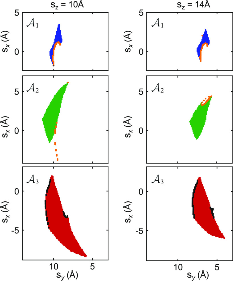
 and
and  ) or black (
 ). Isolated states (prominent in
  ) can only be reached from other (duplicate)
anchor sets (compare Figure 6c).
) can only be reached from other (duplicate)
anchor sets (compare Figure 6c).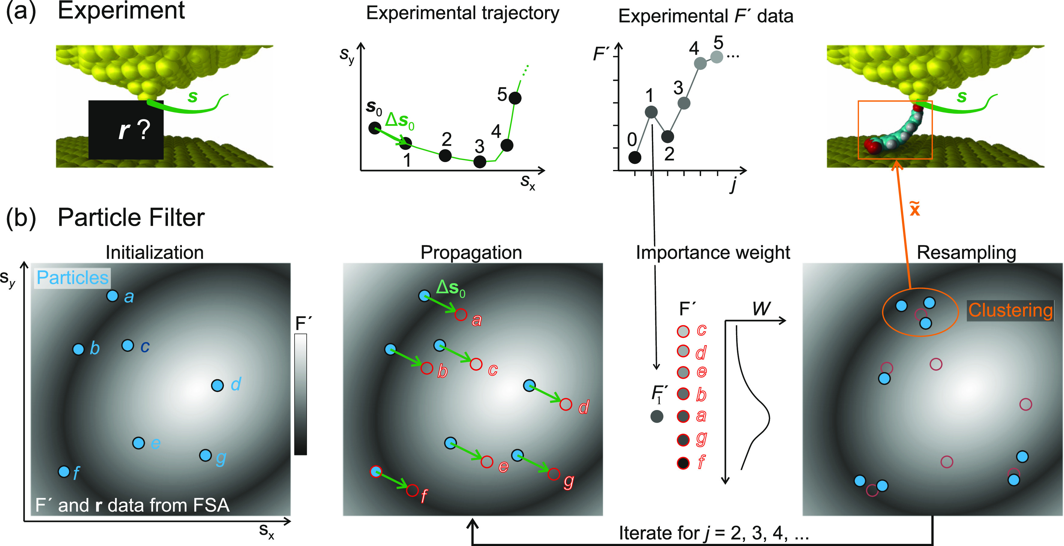
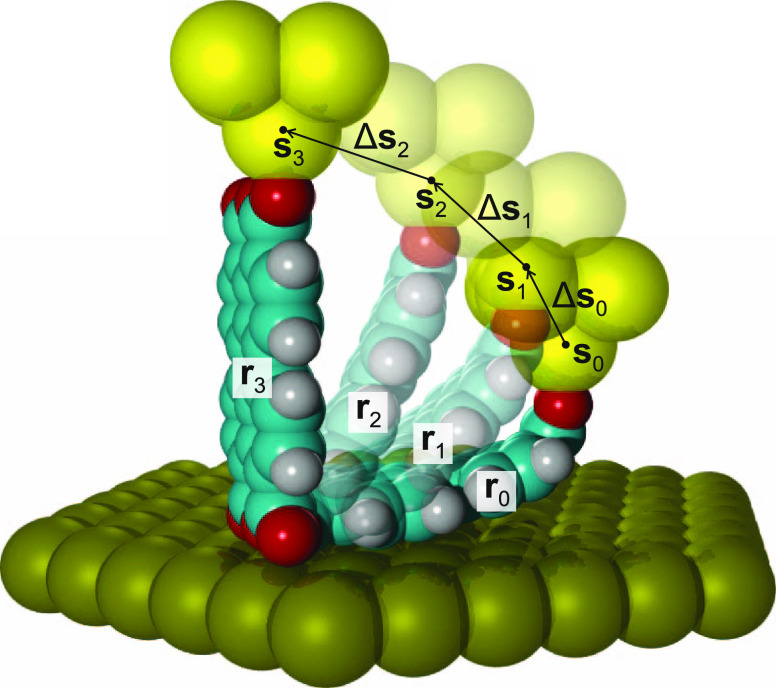
 at random tip–molecule configurations xl, l = 1, ···,
7 (blue). The gray background symbolizes the observation model F′
= U(x) stored in the FSA. (1) Propagation.
All particles are displaced according to the experimental tip displacement
step Δs0 and the state
transition model as xl,1 = S(xl,0, Δs0). Synthetic noise in the displacement
is omitted here. Each particle l has a distinct Fl′ (background greyscale). (2) Importance weight. According to the
agreement between their Fl′ value and the experimental F′, the particles receive individual importance weights Wl (eq 9). (3) Resampling. All particles are randomly
relocated to the proximity of previous particle locations (faint red),
favoring the original locations of particles with high Wl (here: particles a, b, g, and f).
Exploration places a fraction ϵ of the particles in completely
random locations (not shown). (4) Clustering. Regions with high particle
density are identified because they represent the PF’s best
estimates of the actual molecular configuration r1, which is the property of interest. The PF
will iterate through steps (1)–(3) for j =
2, 3, ···, converging the particle locations further
onto good configuration estimates for xj. Step (4) is only required when an
ad hoc conformation estimate x̃ is requested.
at random tip–molecule configurations xl, l = 1, ···,
7 (blue). The gray background symbolizes the observation model F′
= U(x) stored in the FSA. (1) Propagation.
All particles are displaced according to the experimental tip displacement
step Δs0 and the state
transition model as xl,1 = S(xl,0, Δs0). Synthetic noise in the displacement
is omitted here. Each particle l has a distinct Fl′ (background greyscale). (2) Importance weight. According to the
agreement between their Fl′ value and the experimental F′, the particles receive individual importance weights Wl (eq 9). (3) Resampling. All particles are randomly
relocated to the proximity of previous particle locations (faint red),
favoring the original locations of particles with high Wl (here: particles a, b, g, and f).
Exploration places a fraction ϵ of the particles in completely
random locations (not shown). (4) Clustering. Regions with high particle
density are identified because they represent the PF’s best
estimates of the actual molecular configuration r1, which is the property of interest. The PF
will iterate through steps (1)–(3) for j =
2, 3, ···, converging the particle locations further
onto good configuration estimates for xj. Step (4) is only required when an
ad hoc conformation estimate x̃ is requested.


References
-
- Salapaka S. M. Scanning Probe Microscopy. IEEE Control Syst. Mag. 2008, 28, 65–83. 10.1109/MCS.2007.914688. - DOI
LinkOut - more resources
Full Text Sources