Manifold learning for fMRI time-varying functional connectivity

Abstract

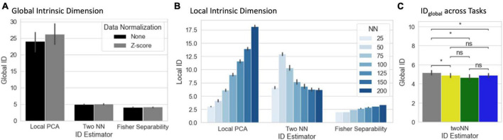
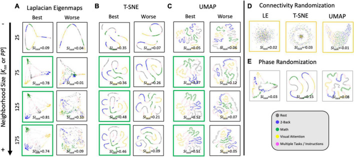
Whole-brain functional connectivity (FC) measured with functional MRI (fMRI) evolves over time in meaningful ways at temporal scales going from years (e.g., development) to seconds [e.g., within-scan time-varying FC (tvFC)]. Yet, our ability to explore tvFC is severely constrained by its large dimensionality (several thousands). To overcome this difficulty, researchers often seek to generate low dimensional representations (e.g., 2D and 3D scatter plots) hoping those will retain important aspects of the data (e.g., relationships to behavior and disease progression). Limited prior empirical work suggests that manifold learning techniques (MLTs)-namely those seeking to infer a low dimensional non-linear surface (i.e., the manifold) where most of the data lies-are good candidates for accomplishing this task. Here we explore this possibility in detail. First, we discuss why one should expect tvFC data to lie on a low dimensional manifold. Second, we estimate what is the intrinsic dimension (ID; i.e., minimum number of latent dimensions) of tvFC data manifolds. Third, we describe the inner workings of three state-of-the-art MLTs: Laplacian Eigenmaps (LEs), T-distributed Stochastic Neighbor Embedding (T-SNE), and Uniform Manifold Approximation and Projection (UMAP). For each method, we empirically evaluate its ability to generate neuro-biologically meaningful representations of tvFC data, as well as their robustness against hyper-parameter selection. Our results show that tvFC data has an ID that ranges between 4 and 26, and that ID varies significantly between rest and task states. We also show how all three methods can effectively capture subject identity and task being performed: UMAP and T-SNE can capture these two levels of detail concurrently, but LE could only capture one at a time. We observed substantial variability in embedding quality across MLTs, and within-MLT as a function of hyper-parameter selection. To help alleviate this issue, we provide heuristics that can inform future studies. Finally, we also demonstrate the importance of feature normalization when combining data across subjects and the role that temporal autocorrelation plays in the application of MLTs to tvFC data. Overall, we conclude that while MLTs can be useful to generate summary views of labeled tvFC data, their application to unlabeled data such as resting-state remains challenging.

Keywords: Laplacian Eigenmaps (LE); T-SNE; Uniform Manifold Approximation and Projection (UMAP); data visualization; fMRI; manifold learning; time-varying functional connectivity.

FIGURE 1

(A) Time-varying FC matrix at scale to illustrate the disproportionate larger dimensionality of the connectivity axis (y-axis) relative to the time axis (x-axis). (B) Same tvFC matrix as in panel (A) but no longer at scale. The x-axis has now been stretched to better observe how connectivity evolves over time. Connections are sorted in terms of their average strength. Task-homogenous windows are clearly marked above the tvFC matrix with color-coded rectangles. (C) Same tvFC matrix with connections sorted in terms of their volatility (as indexes by the coefficient of variance). (D) Same tvFC matrix with connections sorted according to hemispheric membership. Intra-hemispheric connections appear at the top of the matrix and inter-hemispheric at the bottom. Laplacian Eigenmap (correlation distance, k = 90) for the tvFC matrix in panels (A–D) with no color annotation (E), annotated by time (F), and annotated by task (G). (H) Laplacian Eigenmap for the tvFC matrix in panels (A–D) using correlation distance and k = 20. (I) Euclidean distance of each point in the embedding from the origin. Dashed lines indicate automatically detected peaks in the distance trace. Shaded regions around those locations indicate the temporal segments (30 windows) used to compute the FC matrices represented below. (J) FC matrices associated with each scan interval indicated in panel (I). (K) Same information as in panel (J) but shown over a brain surface. Only connections with | r| > 0.4 are shown in these brain maps.

FIGURE 2

The Laplacian Eigenmap algorithm. (A) Representative tvFC matrix for a multi-task run from Gonzalez-Castillo et al. (2015), which consists of a scan acquired continuously as participants engage and transition between four different mental tasks (2-back, math, visual attention (VA), and rest). Additional details in the Dataset portion of the section “Materials and methods.” Columns indicate windows and rows indicate connections. (B) Dissimilarity matrix for the tvFC matrix in panel (A) computed using the Euclidean distance function. (C) Affinity matrix computed for panel (B) using K_nn = 90 neighbors. Black cells indicate 1 (i.e., an edge exists) and white indicate zero (no edge). (D) Graph visualization of the affinity matrix in panel (C). In the top graph all nodes are colored in white to highlight that the LE algorithm used no information about the tasks at any moment. The bottom graph is the same as the one above, but now nodes are colored by task to make apparent how the graph captures the structure of the data (e.g., clusters together windows that correspond to the same experimental task). (E) Final embedding for m = 3. This embedding faithfully presents the task structure of the data. (F) Final embedding for m = 2. In this case, the windows for rest and memory overlap. Red arrows and text indicate decision points in the algorithm. Step-by-step code describing the LE algorithm and used to create the different panels of this figure can be found in the code repository that accompanies this publication (Notebook N03_Figure02_Theory_LE.ipynb).

FIGURE 3

The T-SNE algorithm. (A) Representative tvFC matrix for a multi-task run (same as in Figure 2). Columns indicate windows and rows indicate connections. (B) Dissimilarity matrix for the tvFC matrix in panel (A) computed using the Euclidean distance function. (C) Affinity matrix generated using Eqs 3, 4 and a perplexity value of 100. (D) Random lower-dimensional representation of the data. Each dot represents one column of the data in panel (A). (E) Dissimilarity matrix for the data in panel (D) computed using the Euclidean distance function. (F) Affinity matrix for the data in panel (D) computed using a T-distribution function as in Eq. 5. (G) Evolution of the cost function with the number of gradient descent iterations. In this execution, the early exaggeration factor was set to 4 for the initial 100 iterations [as originally described by van der Maaten and Hinton (2008)]. A dashed vertical line marks the iteration when the early exaggeration factor was removed (early exaggeration phase highlighted in light blue). Below the cost function evolution curve, we show embeddings and affinity matrices for a set of representative iterations. Iterations corresponding to the early exaggeration periods are shown on the left, while iterations for the post early exaggeration period are shown on the right. In the embeddings, points are colored according to the task being performed on each window. Windows that contain more than one task are marked in pink with the label “XXXX.” Step-by-step code describing a basic implementation of the T-SNE algorithm and used to create the different panels of this figure can be found in the code repository that accompanies this publication (Notebook N04_Figure03_Theory_TSNE.ipynb).

FIGURE 4

(A) Input tvFC data (same as in Figure 2). (B) Dissimilarity matrix obtained using the Euclidean distance as a distance function. (C) Binary non-symmetric affinity matrix for K_nn = 90. (D) Graph equivalent of the affinity matrix in panel (C). (E) Effect of the distance normalization step on the original dissimilarities between neighboring nodes. (F) Graph associated with the normalized affinity matrix. (G) Final undirected graph after application of Eq. 15. This is the input to the optimization phase. (H) Representative embeddings at different epochs of the stochastic gradient descent algorithm for an initial learning rate equal to 1. (I) Same as panel (H) but when the initial learning rate is set to 0.01. (J) Difference between embeddings at consecutive epochs measured as the average Euclidean distance across all node locations for an initial learning rate of 1 (dark gray) and 0.01 (light gray). Step-by-step code describing a basic implementation of the UMAP algorithm and used to create the different panels of this figure can be found in the code repository that accompanies this publication (Notebook N05_Figure04_Thoery_UMAP.ipynb).

FIGURE 5

(A) Summary view of global ID estimates segregated by estimation method (local PCA, two nearest neighbors, and Fisher separability) and normalization approach (none or Z-scoring). Bar height corresponds to average across scans, bars indicate 95% confidence intervals. (B) Summary view of local ID estimates segregated by estimation method and neighborhood size (NN = number of neighbors) for the non-normalized data. (C) Statistical differences in global ID across tasks (*p_FDR < 0.05) (gray, rest; yellow, visual attention; green, math; and blue, 2-back).

FIGURE 6

Task separability for single-scan level embeddings. (A) Distribution of SI_task values for original data and null models across all hyperparameters for LE for 2D and 3D embeddings (Total Number of Cases: 20 Subjects × 3 Models × 2 Norm Methods × 3 Distances × 40 Knn values × 2 Dimensions). (B) Same as panel (A) but for T-SNE. (C) Same as panel (A) but for UMAP. (D) SI_task for LE as a function on distance metric and number of final dimensions for the original data. Bold lines indicate mean values across all scans and hyperparameters. Shaded regions indicate 95% confidence interval. (E) Effects of normalization scheme on SI_task at K_nn = 75 for original data and the three distances. (F) Same as panel (D) but for T-SNE. (G) Same as panel (E) but for T-SNE and PP = 75. (H) SI_task dependence on learning rate for T-SNE at PP = 75. (I) Same as panel (D) but for UMAP. (J) Same as panel (E) but for UMAP. (K) Same as panel (H) but for UMAP. In panels (E,G,H,J,K) bar height indicate mean value and error bars indicate 95% confidence interval. Statistical annotations: ^nsnon-significant, *p_Bonf < 0.05, **p_Bonf < 0.01, ***p_Bonf < 0.001, ****p_Bonf < 0.0001.

FIGURE 7

Representative single-scan embeddings. (A) LE embeddings for K_nn = 25,75,125 and 175 generated with the Correlation distance. Left column shows embeddings for the scan that reached the maximum SI_task value across all possible K_nn values. Right column shows embeddings for the scan that reached worse SI_task. In each scatter plot, a dot represents a window of tvFC data (i.e., a column in the tvFC matrix). Dots are annotated by task being performed during that window. (B) T-SNE embeddings computed using the Correlation distance, learning rate = 10 and PP = 25, 75, 125, and 175. These embeddings correspond to the same scans depicted in panel (A). (C) UMAP embeddings computed using the Euclidean distance, learning rate = 0.01 and K_nn = 25, 75, 125, and 175. These also correspond to the same scans depicted in panels (A,C). (D) LE, T-SNE, and UMAP embeddings computed using as input the connectivity randomized version of the same scan corresponding to “best” in panels (A–C). (E) LE, T-SNE, and UMAP embeddings computed using as input the phase randomized version of the same scan corresponding to “best” in panels (A–C).

FIGURE 8

Summary of clustering evaluation for LE group embeddings. (A) Histograms of SI_task values across all hyperparameters when using the Correlation distance with real data. Distributions segregated by grouping method: “Embed + Procrustes” in orange and “Concatenation + Embed” in blue. Dark red outline highlights the section of the distribution for “Embed + Procrustes” that corresponds to instances where more than 3 dimensions were used to compute the Procrustes transformation. (B) Same as panel (A) but this time we report SI_subject instead of SI_task. (C) Group level LE embeddings obtained via “Embed + Procrustes” with an increasing number of dimensions entering the Procrustes transformation step. In all instances we show embeddings annotated by task, including windows that span more than one task and/or instruction periods. For m = 30 we show two additional versions of the embedding, one in which task inhomogeneous windows have been removed, so that task separability becomes clear, and one when windows are annotated by subject identity to demonstrate how inter-individual differences are not captured in this instance. (D) Representative group embedding with high SI_subject obtained via “Concatenation + Embed” approach.

FIGURE 9

Summary of clustering evaluation for UMAP group embeddings. (A) Histograms of SI_task values across all hyperparameters when using Euclidean distance on real data. Distributions are segregated by grouping method: “Embed + Procrustes” in orange and “Concatenation + Embed” in blue. Dark orange outline highlights the section of the “Embed + Procrustes” distribution that corresponds to instances where more than 3 dimensions were used to compute the Procrustes transformation. (B) Histograms of SI_subject values across all hyperparameters when using Euclidean distance on real data. Distributions are segregated by grouping method in the same way as in panel (A). Light blue contour highlights the part of the distribution for “Concatenation + Embed” computed on data that has been normalized (e.g., Z-scored), while the dark blue contour highlights the portion corresponding to data that has not been normalized. (C) High quality group-level “Embed + Procrustes” embedding annotated by task (left) and subject identity (right). (D) High quality group-level “Concatenation + Embed” annotated by task (left) and subject identity (right).

FIGURE 10

Summary of predictive framework evaluation for LE (A,C) and UMAP (B,D) group embeddings using the split-half cross validation scheme. (A) Classification accuracy as a function of the number of LE dimensions used as input features to the logistic regression classifier. Classification improves as m increases up to m = 20. (B) Classification accuracy as a function of the number of UMAP dimensions used as input features to the logistic regression classifier. Classification improves as m increases up to m = 5. Statistical annotations for panels (A,B) as follows: ^nsnon-significant, **p_Bonf < 0.01, ***p_Bonf < 0.001, ****p_Bonf < 0.0001. (C) Average coefficients associated with each LE dimension for classifiers trained using m = 30 dimensions. For each m value, we stack the average coefficients associated with each label, which are colored as follows: blue, 2-back; green, math; yellow, visual attention; gray, rest. (D) Same as panel (C) but for UMAP.

References

1. Albergante L., Bac J., Zinovyev A. (2019). Estimating the effective dimension of large biological datasets using Fisher separability analysis. arXiv [Preprint]. 10.1109/ijcnn.2019.8852450 - DOI
1. Allen E., Damaraju E., Plis S., Erhardt E. (2014). Tracking whole-brain connectivity dynamics in the resting state. Cereb. Cortex 24 663–676. 10.1093/cercor/bhs352 - DOI - PMC - PubMed
1. Amsaleg L., Bailey J., Barbe D., Erfani S., Houle M. E., Nguyen V., et al. (2017). “The Vulnerability of Learning to Adversarial Perturbation Increases with Intrinsic Dimensionality,” in Proceedings of the IEEE Workshop on Information Forensics and Security, Manhattan, NY, 10.1109/wifs.2017.8267651 - DOI
1. Ansuini A., Laio A., Macke J. H., Zoccolan D. (2019). “Intrinsic dimension of data representations in deep neural networks,” in Proceedings of the Advances in Neural Information Processing Systems, Red Hook, NY.
1. Bac J., Mirkes E. M., Gorban A. N., Tyukin I., Zinovyev A. (2021). Scikit-dimension: A python package for intrinsic dimension estimation. Entropy 23:1368. 10.3390/e23101368 - DOI - PMC - PubMed
LinkOut - more resources