Beyond Correlation: Optimal Transport Metrics For Characterizing Representational Stability and Remapping in Neurons Encoding Spatial Memory

Abstract

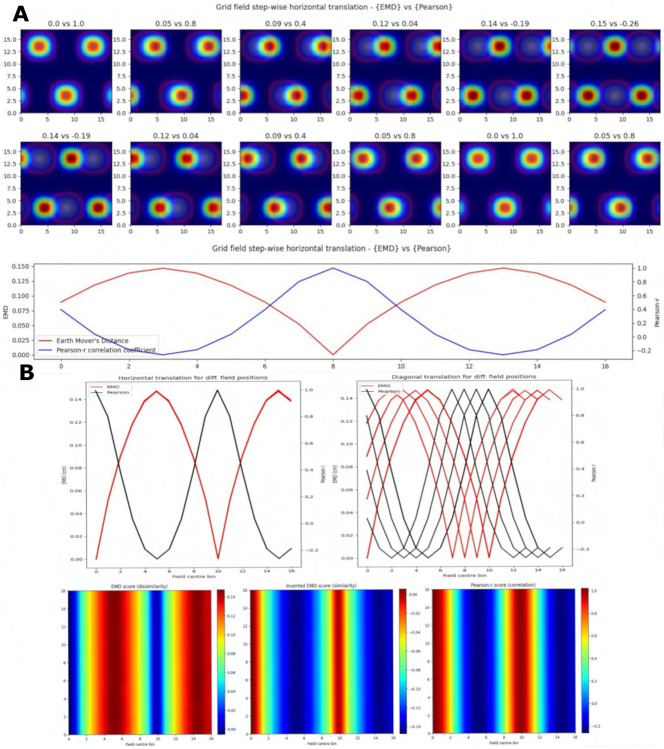
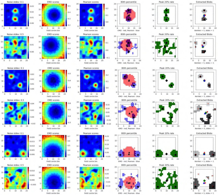
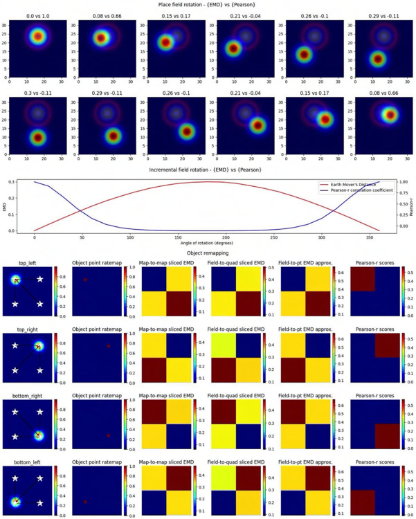
Spatial representations in the entorhinal cortex (EC) and hippocampus (HPC) are fundamental to cognitive functions like navigation and memory. These representations, embodied in spatial field maps, dynamically remap in response to environmental changes. However, current methods, such as Pearson's correlation coefficient, struggle to capture the complexity of these remapping events, especially when fields do not overlap, or transformations are non-linear. This limitation hinders our understanding and quantification of remapping, a key aspect of spatial memory function. To address this, we propose a family of metrics based on the Earth Mover's Distance (EMD) as a versatile framework for characterizing remapping. Applied to both normalized and unnormalized distributions, the EMD provides a granular, noise-resistant, and rate-robust description of remapping. This approach enables the identification of specific cell types and the characterization of remapping in various scenarios, including disease models. Furthermore, the EMD's properties can be manipulated to identify spatially tuned cell types and to explore remapping as it relates to alternate information forms such as spatiotemporal coding. By employing approximations of the EMD, we present a feasible, lightweight approach that complements traditional methods. Our findings underscore the potential of the EMD as a powerful tool for enhancing our understanding of remapping in the brain and its implications for spatial navigation, memory studies and beyond.

Keywords: activity maps; grid cell; optimal transport; place cell; remapping; spatial coding; spatiotemporal; stability.

Figure 1.. Identical place field translation.

Stepwise horizontal linear translation of identical, overlapping place fields (N = 17, σ = 3) moving from the center to the right (A, C). EMD score is shown on the left while Pearson’s r is shown on the right (top panel - EMD vs Pearson). 12 steps are shown and scores are rounded for display. Scores from remapping tested at all possible centroids along a single row on the rate map (bottom panel). EMD and Pearson’s r scores tested at all possible centroids in the rate map (N*N) (B, D). Scores for horizontal and diagonal translations along the rate map are shown for all rows (N = 17) (top panel). Heatmap showing the gradient of scores for both raw and inverted EMD (left and center) and for Pearson’s r (right) (bottom panel).

Figure 1.. Identical place field translation.

Stepwise horizontal linear translation of identical, overlapping place fields (N = 17, σ = 3) moving from the center to the right (A, C). EMD score is shown on the left while Pearson’s r is shown on the right (top panel - EMD vs Pearson). 12 steps are shown and scores are rounded for display. Scores from remapping tested at all possible centroids along a single row on the rate map (bottom panel). EMD and Pearson’s r scores tested at all possible centroids in the rate map (N*N) (B, D). Scores for horizontal and diagonal translations along the rate map are shown for all rows (N = 17) (top panel). Heatmap showing the gradient of scores for both raw and inverted EMD (left and center) and for Pearson’s r (right) (bottom panel).

Figure 2.. Identical grid field translation.

Stepwise horizontal linear translation of identical, overlapping grid fields (N = 3, σ = 1) moving from the top left corner to the right and/or downwards on a rate map (N = 17) (A, C) EMD score is shown on the left while Pearson’s r is shown on the right. 12 steps are shown and scores are rounded for display (top panel - EMD vs Pearson). Grid maps were sliced from a larger map with sufficient fields and bins to support N*N steps. Initial grid maps were chosen by taking a slice from the wider map. Scores from remapping tested across N*N different shifts from the initial grid map (0 to N combinations) (bottom panel). EMD and Pearson’s r scores tested at N*N different centroid positions on the wider grid (B, D). Scores for horizontal and diagonal translations along the rate map are shown for all rows (N = 17) (top panel). Heatmap showing the gradient of scores for both raw and inverted EMD (left and center) and for Pearson’s r (right) (bottom panel).

Figure 2.. Identical grid field translation.

Stepwise horizontal linear translation of identical, overlapping grid fields (N = 3, σ = 1) moving from the top left corner to the right and/or downwards on a rate map (N = 17) (A, C) EMD score is shown on the left while Pearson’s r is shown on the right. 12 steps are shown and scores are rounded for display (top panel - EMD vs Pearson). Grid maps were sliced from a larger map with sufficient fields and bins to support N*N steps. Initial grid maps were chosen by taking a slice from the wider map. Scores from remapping tested across N*N different shifts from the initial grid map (0 to N combinations) (bottom panel). EMD and Pearson’s r scores tested at N*N different centroid positions on the wider grid (B, D). Scores for horizontal and diagonal translations along the rate map are shown for all rows (N = 17) (top panel). Heatmap showing the gradient of scores for both raw and inverted EMD (left and center) and for Pearson’s r (right) (bottom panel).

Figure 3.. Incremental field degeneration.

Stepwise nonlinear translation of overlapping fields (N = 33) relative to a fixed field at σ = 3. 12 steps are shown with 6 scaling down and 6 scaling up relative to the fixed field (A). EMD score is shown on the left while Pearson’s r is shown on the right (left panel). Scores from remapping tested across a range of standard deviations for the scaling field (right panel). Incremental field degeneration for a pair of fields, non-overlapping and overlapping (B,C). Left panels show the stepwise degradation in the rate map due to randomly sampled normally distributed noise with varying standard deviations. Noise standard deviations are shown above the rate map plots. The distribution plots show the computed remapping score between the pair of fields for the overlapping and non-overlapping cases. Both cases have values for the EMD (red), field EMD (green) and Pearson’s r scores (blue) displayed (right panels).

Figure 4.. Single field localization.

Field localization plots across two different noise levels (rows: low noise 0.1 and high noise 0.5). For each row in a plot, the first column shows the ratemap post added noise with padding, smoothing and normalizing. The second column shows the EMD distribution on the padded rate map with scores being relative to a point map with all the density placed in the bin at which the EMD score is found. The third column shows the same map to point computation for Pearson’s r scores. The fourth column shows the 80th percentile scores for the EMD (red) and Pearson’s r distributions (blue). The fifth column shows the top 20% firing rates in the cell. The last column (sixth) holds the extracted blobs (fields) from the padded ratemap with the centroid of each blob shown in red. The circle represents the true field centroid. The star represents the centroid computed on the peak EMD scores. The triangle is the centroid computed from the peak Pearson’s r scores. The diamond is the centroid from the peak firing rates. The red dots are the centroids of a given field

Figure 5.. Dual field localization.

Field localization plots across two different noise levels (rows: low noise 0.1 and high noise 0.5). For each row in a plot, the first column shows the ratemap post added noise with padding, smoothing and normalizing. The second column shows the EMD distribution on the padded rate map with scores being relative to a point map with all the density placed in the bin at which the EMD score is found. The third column shows the same map to point computation for Pearson’s r scores. The fourth column shows the 80th percentile scores for the EMD (red) and Pearson’s r distributions (blue). The fifth column shows the top 20% firing rates in the cell. The last column (sixth) holds the extracted blobs (fields) from the padded ratemap with the centroid of each blob shown in red. The circle represents the true field centroid. The star represents the centroid computed on the peak EMD scores. The triangle is the centroid computed from the peak Pearson’s r scores. The diamond is the centroid from the peak firing rates. The red dots are the centroids of a given field

Figure 6.. Complex non-linear field remapping.

Stepwise nonlinear translation of overlapping fields (N = 33) relative to a fixed field at σ = 3. 12 steps are shown with 6 scaled down and 6 scaled up relative to the fixed field (A). EMD score is shown on the left while Pearson’s r is shown on the right (top panel). Scores from remapping tested across a range of rotation angles (bottom panel). Four corner point driven remapping with top left, top right, bottom right and bottom left tested. Fields were positioned so as to be fully encompassed by the rate map area. The first column shows the field location, four possible object/point/stimulus locations (stars), and distances from the field centroid to each of the four positions. The second column shows the whole map to whole map EMD scores with the full rate map and a pointmap (1 at object location, 0 everywhere else). The third shows a field restricted EMD between a field and a quadrant of multiple bins. The fourth column shows an approximation to the whole map sliced EMD using only the field and the single point object point (single point Wasserstein). The last column holds the Pearson’s r scores. Heatmaps demonstrate the scores in the four possible corners.

Figure 7.. EMD robustness to intensity changes.

Incremental field scaling (increasing intensity) across a (17,17) ratemap with a field at the center (A). Field is scaled from = 1 to σ = 6 (left). Intensity changes are considered using whole map EMD (red), field restricted EMD (green) and a binary EMD (blue) using raw spike positions. Normalized (top right panel) and unnormalized (bottom right panel) weights are shown for both. EMD scores tested against different firing rate ratios for two identical fields (B). Ratios greater than 1 and less than 1 were tested.

Figure 8.. Individual cell examples.

Examples of ratemaps from the MEC and HPC of AD mouse models for a reference session and a shifting session. Gradient of Pearson’s r scores tested at all possible map shift centers (N*N) is shown to the far right of each cell example with the EMD gradient immediately to the left of it. For each MEC example, the top row demonstrates a shift with no wrap (0 padding) while the bottom row demonstrates a shift with wrapping (A). For each HPC example, only the no wrap row is provided, and examples of matched cells across circular to rectangular arena transitions are included (B).

Figure 9.. Place cell population decoding.

Place cell population decoding using a reference template and a population of 1D rates across a 200cm linear track. The first plot in a row shows a population map of linear firing rates. The second plot shows the distribution of EMD values, and the running average. The third plot shows the population of correlation values, and the running average. The last plot shows the peak firing rate trend overlaid with the running averages of each score distribution. Two sets of examples are provided with reference templates highest in density at the start (A) and in the center (B). In each set, the first row of plots uses a reference map with all the activity in a single bin. The second row uses a map with the activity spread out across 10 bins. The last row uses a 1D gaussian template with sigma = 5. Reference points, and windows, are plotted with a dashed black line in the final plot of each row. Reference gaussians are overlaid in the final plot of each row. Population decoding with quantiles instead of distances. Quantiles are computed using the distribution of EMD distances from all other cells (C). Quantiles are computed using the distribution of EMD distances from a given cell relative to random reference locations (D).

References

1. Anderson M. I. and Jeffery K. J. (2003). Heterogeneous modulation of place cell firing by changes in context 23, 8827–8835. doi:10.1523/JNEUROSCI.23-26-08827.2003. Publisher: Society for Neuroscience Section: Behavioral/Systems/Cognitive - DOI - PMC - PubMed
1. Bonneel N., Rabin J., Peyré G., and Pfister H. (2015). Sliced and radon wasserstein barycenters of measures 51, 22–45. doi:10.1007/s10851-014-0506-3 - DOI
1. Bonnevie T., Dunn B., Fyhn M., Hafting T., Derdikman D., Kubie J. L., et al. (2013). Grid cells require excitatory drive from the hippocampus 16, 309–317. doi:10.1038/nn.3311. Number: 3 Publisher: Nature Publishing Group - DOI - PubMed
1. Bostock E., Muller R. U., and Kubie J. L. (1991). Experience-dependent modifications of hippocampal place cell firing 1, 193–205. doi:10.1002/hipo.450010207. _eprint: https://onlinelibrary.wiley.com/doi/pdf/10.1002/hipo.450010207 - DOI - DOI - PubMed
1. Brandon M. P., Bogaard A. R., Libby C. P., Connerney M. A., Gupta K., and Hasselmo M. E. (2011). Reduction of theta rhythm dissociates grid cell spatial periodicity from directional tuning 332, 595–599. doi:10.1126/science.1201652. Publisher: American Association for the Advancement of Science - DOI - PMC - PubMed
Publication types