A dual Purkinje cell rate and synchrony code sculpts reach kinematics

Abstract

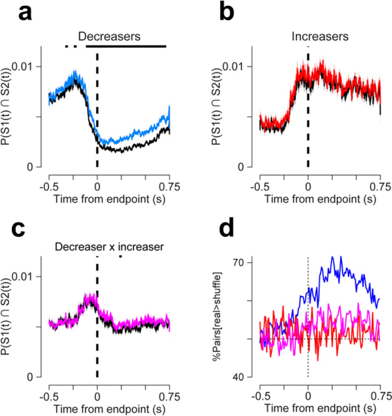
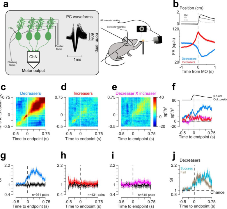
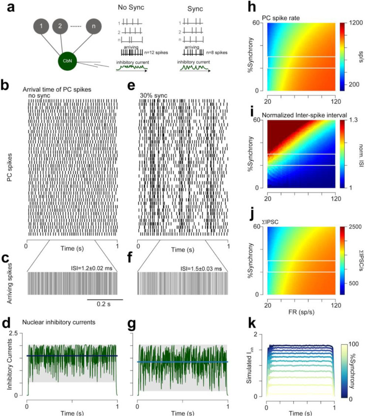
Cerebellar Purkinje cells (PCs) encode movement kinematics in their population firing rates. Firing rate suppression is hypothesized to disinhibit neurons in the cerebellar nuclei, promoting adaptive movement adjustments. Debates persist, however, about whether a second disinhibitory mechanism, PC simple spike synchrony, is a relevant population code. We addressed this question by relating PC rate and synchrony patterns recorded with high density probes, to mouse reach kinematics. We discovered behavioral correlates of PC synchrony that align with a known causal relationship between activity in cerebellar output. Reach deceleration was positively correlated with both Purkinje firing rate decreases and synchrony, consistent with both mechanisms disinhibiting target neurons, which are known to adjust reach velocity. Direct tests of the contribution of each coding scheme to nuclear firing using dynamic clamp, combining physiological rate and synchrony patterns ex vivo, confirmed that physiological levels of PC simple spike synchrony are highly facilitatory for nuclear firing. These findings suggest that PC firing rate and synchrony collaborate to exert fine control of movement.

Extended Data Figure 1:

Synchrony index averaged across mice for all pPCs (a-c) and for confirmed PCs (d-f). (a) Left, average SI for decreasers calculated across 7 mice. Right, average SI in the time window between −0.3 and 0.3 s of the reach for each mouse (dots) (paired t-test; p<0.05 compared to shuffled data). (b) Same as a) for increasers (p=0.1). (c) Same as a) for mixed pairs (p=0.52). (d-f) SI of complex spike-confirmed PCs that decrease their firing (d;n=37 pairs) increase their firing (e;n=17 pairs) or decrease vs. increase pairs (f, n=3 pairs), relative to shuffled data (black).

Extended Data Figure 2:

Probability of coincident spikes between pPCs. (a) Co-firing of pPCs across time relative to reach endpoint. Co-firing (colored traces) was calculated as the probability of sampling two spikes simultaneously from two cells in a 1-ms time bin (not corrected for average firing rate). Black curves report co-firing in shuffled data. Asterisks above show timepoints which were statistically significantly different from shuffle (paired t-test; p<4×10⁻⁵; Bonferroni corrected for multiple testing). (b) Same as a, but for increasers. (c) Same as a, but for pairs of increasers vs decreasers. (d) The percentage of pairs that exhibit higher co-firing relative to shuffled data, as a function of time from reach endpoint.

Extended Data Figure 3:

Data simulations to test sensitivity of synchrony index to firing rate. (a) Average simulated firing rate of simulated PCs that decrease rates. The simulation (see methods) was made for 500 pairs of decreasers, with 60 trials. (b) Average (±s.e.m.) synchrony index of the simulated data. (c) jPETH of the simulated data. (d) Average diagonal of the jPETH matrix in c. (e) The synchrony index after artificially synchronizing the firing of simulated pairs in the time window between 0 and 0.5 s. (f) The average SI (between 0 and 0.5s) from panel e (from 0% to 100% spike synchrony: 1±0.002; 3.9±0.01; 6±0.02; 7.6±0.02; 8.9±0.03). (g) From left to right, the jPETH for the different synchronization levels (0, 25, 50, 75 and 100%) in the time window between 0 and 0.5 s.

Extended Data Figure 4:

Relationship between synchrony and movement kinematics in confirmed PCs. (a) For each session the SI was calculated between different pairs for trials with fastest (green) or slowest (purple) decelerations. Points on top correspond to time points where the two traces have significant difference (p<4×10–5 Bonferroni corrected for multiple testing). Inset show magnification of the difference between the two conditions in the time leading to endpoint. (b) The maximal deceleration observed for trials with the highest SI (orange) or trials with the lowest SI (blue) in the outward (Out.) or vertical (Up.) position (n=37 pairs. Out.: Low SI: 177.4±38.1 cm/s²; High SI: 403.6±46 cm/s²; Kolmogrov-Smirnov test; p=8.2×10⁻³³; Up.: Low SI: 213.3±48.2 cm/s²; High SI: 598.1±76.3 cm/s²; p=1.9×10⁻⁵). (c) For each session the SI was calculated between different pairs for trials with hypermetric (overshoot; green) or hypometric (undershoot; purple) reach endpoints. Points on top correspond to time points where the two traces have significant difference (p<4×10⁻⁵ Bonferroni corrected for multiple testing). Inset show magnification of the difference between the two conditions in the time leading to endpoint. (d) Correlation between the sum of the SI per trial and the endpoint changes (mean±s.e.m.; −0.25±0.02; p=2×10⁻¹²; t-value=10.5; dof=36; Cohen’s D= 1.7). (e) Endpoint locations for trials with the highest SI (orange), and trials with the lowest SI (blue), per cell pair (n=37 pairs; High SI: Δout: −0.07±0.012 cm; Δup: −0.04±0.013 cm; Low SI: Δout: −0.03±0.013 cm; Δup: 0.01±0.02 cm; Wilcoxon’s signed rank; p<3.5×10⁻⁵; r=0.68;Wilcoxon’s signed rank). (f) The change in the outward (Out.) or vertical (Up.) endpoint position for low SI and high SI trials (Kolmogrov-Smirnov test; Δout: p-value= 1.7×10⁻⁶;D= 0.6; Δup: p-value= 0.11; D= 0.27; ΔEuc: Low=0.032±0.02 to high: −0.08±0.02; p-value= 1.9×10⁻⁵;D= 0.54).

Extended Data Figure 5:

jPETHs of reaches segregated by endpoint. (a-b) jPETH matrices for the top (a) and bottom (b) quartiles of endpoint position, aligned to time of endpoint (white lines). (c) Co-firing computed along the diagonals of the jPETHs, showing average (±s.e.m.) for the hypometric (undershoot, purple) and hypermetric (overshoot, green) reaches. (d) The integral of the co-firing for the shaded area in c (Wilcoxon’s signed-rank; p=2.7×10⁻⁷; r=0.17).

Extended Data Figure 6:

Statistics relating PC rate modulation and SI to behavioral variables (associated with data in Fig. 3a and 3b) (a) Surprise values (−log(p-value)) of the heatmap seen in Fig. 3a relative to 1,000 randomly shuffled matrices. Darker hues correspond to higher surprise and lower p-values. (b) The distribution of the bins that are located above (red) or below (blue) the main diagonal of the heatmap in 3a (under: 0.04±0.0008; above: 0.07±0.004; Wilcoxon’s ranked sum; p<7.3 ×10⁻¹²; r= 0.92). (c) same as a), but for the data seen in Fig. 3b. (d) The distribution of the bins that are located above (orange) or below (blue) the main diagonal of the heatmap in 3b (under: −0.012±0.002; above: −0.038±0.003; Wilcoxon’s ranked sum; p<9.6×10⁻¹⁰; r=0.82).

Figure 1:

Dynamics of simple spike synchrony during reaching. (a) In head-fixed mice, neuropixels recordings were made from Lobules 4/5 and simplex while the mice performed reaching towards food pellets. Right panel shows the average normalized waveforms for units classified as Purkinje cells. (b) Top: average hand position in the outward, upward and lateral axes around time of motion onset (dashed line). Bottom: average (±s.e.m) firing rates of PCs/putative PCs (pPCs) around time of threshold crossing. Blue trace shows the average firing for the decreasers and red for the increasers. Shaded areas are the standard error of the mean (s.e.m.). (c) Joint peri-event time histogram (jPETH; see methods) calculated between the decreasers. Straight white lines indicate the time of endpoint; n=951 pairs. (d) Same as c, for increasers, n=431 pairs. (e) Same as c, for mixed pairs, n=515 pairs. (f) Matrix diagonals from jPETHs in c-e summarize the coordinated firing across the reach. Blue- Decreasers, red- increasers and magenta- mixed. The black line in top panel corresponds to the hand outward position. (g) Synchrony index (SI) between simultaneously recorded Purkinje cells during reaching around time of endpoint (dashed line). Black lines indicate the SI calculated when the trials were shuffled and blue line is the average SI for the real data, shaded areas around traces correspond to s.e.m.. (h) similar to g for increasers (red). (i) similar to g, but for pairs consisting of one decreaser and one increaser (magenta). (j) The SI between decreasers for either successful (blue) or failed (gray) trials around endpoint position.

Figure 2:

Relationship between SI and behavioral kinematics. (a) For each session, the SI was calculated between different pairs for trials with fastest (green) or slowest (purple) decelerations.Insets show magnification of the difference between the two conditions in the time leading to endpoint (Average (±s.e.m.) SI in times −0.3 to 0s around the endpoint; Slow: 1.07± 0.02; Fast: 1.13±0.02; Wilcoxon’s signed rank; p=0.02; r=0.08). (b) The maximal deceleration observed for trials with the highest SI (orange; calculated for the 0.3 s preceding endpoint time) or trials with the lowest SI (blue) in the outward (Out.) or vertical (Up.) position (n=951 pairs. Out.: Low SI: 227.2±11.9 cm/s²; High SI: 316.5.4±14.4 cm/s²; Kolmogrov-Smirnov test: p=5.7×10⁻⁹; Up.: Low SI: 201.5±11.5 cm/s2; High SI: 297.8±12.7 cm/s²;p=6.2×10⁻¹⁴). (c) For each session the SI was calculated between different pairs for trials with hypermetric (overshoot; green) or hypometric (undershoot; purple) reach endpoints. Points on top correspond to time points where the two traces have significant difference (p<0.05). Inset shows magnification of the difference between the two conditions in the time leading to endpoint. (d) Correlation between the sum of the SI per trial and the endpoint changes (mean±s.e.m.; −0.09±0.007; p=4.2×10⁻³⁵; r=0.4). (e) Endpoint locations for trials with the highest SI (orange), and trials with the lowest SI (blue), per pair of cells (n=951 pairs; Low SI: Δout: 0.016±0.003 cm; Δup: 0.03±0.004 cm; High SI: Δout: −0.033±0.003 cm; Δup: −0.04±0.003 cm; Wilcoxon’s signed rank; p=1.2×10⁻⁴⁸; r=0.48). Also shown is the distribution of the outward (bottom) or upward (left) endpoint position per condition. (f) The change in the outward (Out.), vertical (Up.) or Euclidean (Euc) endpoint position for low SI (blue) and high SI (orange) trials (Kolmogrov-Smirnov test; Δout: p=1.4×10⁻²¹; Δup: p=5.4×10⁻²¹; Euc.: Low SI: 0.027±0.004, High SI: −0.047±0.003, p=8.2×10⁻²⁴).

Figure 3:

Synchrony and rate modulation jointly influence movement kinematics. (a) Heatmap showing the average deceleration as a function of SI (y-axis) and modulation changes (x-axis). The SI and Modulation were calculated for time window of −0.3 to 0.3 s around the endpoint position to capture the whole movement and normalized on a session basis. The deceleration was also normalized per session to avoid behavioral variability between sessions and mice. (b) Same as (a), for the relationship between the SI, the modulation and the reach endpoint, difference in endpoint position was calculated as the change in trial-by-trial endpoint position from the average endpoint for a session. (c) Change of deceleration (dec, top) and endpoint (end; bottom) as function of changing Modulation (green), changing SI (purple; Note that the SI axis is reversed) or both (calculated from the antidiagonal of the matrices in a-b (orange. The slope of each scatter is shown. (d) Same as a, for the relationship between the SI, rate modulation, and reach success rate.

Figure 4:

Nuclear response to PC firing simulation. (a) schematics of the model. Nuclear cell (Nu) receive input from n PCs (n=40). When there is not synchrony, the number of spikes that arrive at the Nu is the same as the total number of spikes for all the converging PCs (“arriving”), however, when synchronized, spikes superimpose, such that >1 spikes can arrive at the same time at the Nu, eliciting short and one IPSC, such that the total number of arriving spikes is lower than that of the total spike number that was fired by the PCs. (b) example of non-synchronized PC firing, for 40 cells. (c) the train of spikes that arrive at the CbN, each line correspond to ≥1 spikes at the specific time bin. The average inter-spike interval (ISI) value ± s.e.m. is shown above the trace (d) the simulated Nu inhibitory currents elicited by the PC spikes. Each spike elicited an IPSC with normalized amplitude 1 and τ =2.5ms (40 sp/s firing rate). Bold line shows the average current and gray shaded area the range of currents observed. (e) Same as b, for 30% synchronized spiking. (f) same as c, for synchronized spiking. (g) same as d, for synchronized spiking (30% synchrony). (h) The number of spikes that arrive at the Nu, as a function of the synchrony % for different baseline firing of the PCs (n=40 converging cells). The data represent 1,000 iterations of the model. White lines show the range of synchrony levels that are observed in vivo. (i) The average inter-spike interval (ISI) observed by the Nu cell given the different FR and synchrony level. (j) The integral of the inhibitory currents (see d) as a function of increasing synchrony and different firing frequencies. (k) the average change in inhibitory current as a function of the synchrony increase for 40 converging PCs firing at 40 sp/s. Same as d and g, for 1,000 iterations.

Figure 5:

Synchrony and rate are required for eliciting nuclear firing in vitro. (a) Schematics showing the dynamic clamp experiment setup. (b) Nuclear response to simulated PC trains. From top to bottom: PC pool peri-event time histogram (PETHs) used to construct IPSCs trains (from Calame et al.), example traces of nuclear cell response to each pool, and mean nuclear response (mean±s.e.m.; n=13 cells). (c) Nuclear cell responses to pooled PCs (black) with synchrony (blue) as derived from our in vivo measurements. Middle panel shows representative voltage traces for responses to non-synchronized (black) and synchronized (blue) PC pools. Bottom panel shows the mean nuclear response (± s.e.m.) to the PC activity with (blue) or without (black) synchrony. (d). Summary data for peak nuclear responses. Mean nuclear peak rate when the 2 PC trains had no applied synchrony (no sync; from b; 9.57±2.87, 10.5±3.32, and 12.6±3.28 sp/s, respectively, 1 way ANOVA F=0.23, p=0.79 compared to the nuclear response with applied synchrony (no sync:11.2±3.6 sp/s. sync: 27.1±3.5 sp/s; paired t-test: p=3×10⁻⁶; n=10 cells). (e) Representative traces of nuclear responses to PC pools held at a fixed mean rate in 10 sp/s intervals, while synchrony (blue trace) was increased throughout the trace. (f) normalized nuclear response to PC pools with a static rate between 40 and 100 sp/s, and SI of either 1.5 or 2 (n=10 cells; Two-ways ANOVA; F₆(PC firing)=5.15, p=1×10⁻⁴; F₁(SI)=15.62, p=1.4×10⁻⁴). (g) Heatmap showing the change in the nuclear response as a function of PC rate (x-axis) and SI (y-axis).

References

1. Bastian A. J., Martin T. A., Keating J. G. & Thach W. T. Cerebellar ataxia: Abnormal control of interaction torques across multiple joints. J. Neurophysiol. 76, 492–509 (1996). - PubMed
1. Nashef A., Mitelman R., Harel R., Joshua M. & Prut Y. Area-specific thalamocortical synchronization underlies the transition from motor planning to execution. Proc. Natl. Acad. Sci. U. S. A. 118, (2021). - PMC - PubMed
1. Nashef A., Cohen O., Harel R., Israel Z. & Prut Y. Reversible Block of Cerebellar Outflow Reveals Cortical Circuitry for Motor Coordination. Cell Rep. 27, 2608–2619.e4 (2019). - PubMed
1. Nashef A., Cohen O., Israel Z., Harel R. & Prut Y. Cerebellar Shaping of Motor Cortical Firing Is Correlated with Timing of Motor Actions. Cell Rep. 23, 1275–1285 (2018). - PubMed
1. Gao Z. et al. A cortico-cerebellar loop for motor planning. Nature 563, 113–116 (2018). - PMC - PubMed
Publication types