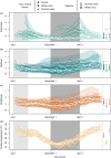
Remotely sensed environmental measurements detect decoupled processes driving population dynamics at contrasting scales

Abstract

The increasing availability of satellite imagery has supported a rapid expansion in forward-looking studies seeking to track and predict how climate change will influence wild population dynamics. However, these data can also be used in retrospect to provide additional context for historical data in the absence of contemporaneous environmental measurements. We used 167 Landsat-5 Thematic Mapper (TM) images spanning 13 years to identify environmental drivers of fitness and population size in a well-characterized population of banner-tailed kangaroo rats (Dipodomys spectabilis) in the southwestern United States. We found evidence of two decoupled processes that may be driving population dynamics in opposing directions over distinct time frames. Specifically, increasing mean surface temperature corresponded to increased individual fitness, where fitness is defined as the number of offspring produced by a single individual. This result contrasts with our findings for population size, where increasing surface temperature led to decreased numbers of active mounds. These relationships between surface temperature and (i) individual fitness and (ii) population size would not have been identified in the absence of remotely sensed data, indicating that such information can be used to test existing hypotheses and generate new ecological predictions regarding fitness at multiple spatial scales and degrees of sampling effort. To our knowledge, this study is the first to directly link remotely sensed environmental data to individual fitness in a nearly exhaustively sampled population, opening a new avenue for incorporating remote sensing data into eco-evolutionary studies.

Keywords: Landsat; fitness; monitoring; population dynamics.

FIGURE 1

(a) Map of the area surrounding the study site, which is situated in Arizona near the New Mexico and Mexico borders. The site is located just southeast of the Chiricahua Mountains. (b) Map of the study site with all mounds included in this study marked with points. The mounds are located on primarily flat areas surrounding a cinder cone.

FIGURE 2

Schematic showing temporal alignments between the predictor and response variables tested in the study. For example: annual means used to predict the number of offspring produced in year t were calculated from environmental data collected from July, year t − 1 through June, year t, whereas winter rainy season means were calculated from data collected from December, year t − 1 through March, year t. Although not indicated in this figure, PRISM data were only used as predictor variables for population fitness and number of active mounds (i.e., not for measures of individual fitness). Summer and winter rainy season results are indicated by “S” and “W,” respectively.

FIGURE 3

Mean values of Tasseled Cap indices (a–c) and surface temperature (d) across days of the year. Means were calculated using all cells that were occupied in at least 1 year over the course of the study plus all cells directly adjacent to those occupied cells. Note that the x‐axes are offset such that the axis begins with July 1 and ends with June 30. White lines connect dates from July 1 in each year through June 30 in the subsequent year. Vertices for shaded polygons encompass one standard deviation around each mean. The points to the right of the dashed line indicate annual and rainy season mean values within each year.

FIGURE 4

Schematic summarizing the statistically significant relationships identified between environmental variables and fitness or population size. “S” and “W” indicate summer and winter rainy season results, respectively. The sign in each colored polygon indicates the direction of the relationship (i.e., the only negative relationship identified was between mean annual surface temperature and number of active mounds). Polygon color indicates environmental predictor variable with outline pattern indicating the scale at which variables were tested (i.e., individual and population fitness and population size).

FIGURE 5

(a–c) Significant positive relationships between surface temperature and measures of individual fitness. Panels a and b present the effects of mean annual and mean winter rainy season surface temperatures, respectively, on number of offspring produced by individual females while setting the non‐focal predictor variable in each negative binomial model equal to its mean value. Panel c presents the final negative binomial model predicting number of surviving offspring with mean annual surface temperature. (d) Linear regression describing negative effect of mean annual surface temperature on population size, as measured by number of active mounds. For all panels, shaded polygons represent 95% confidence intervals. Statistical results for models are presented in Tables 1, 2, 3, 4 and Table A2.

FIGURE A1

Temporal distribution of retained Landsat 5 scenes (n = 167) across rainy seasons and meteorological seasons used for equalizing means within each year. Note that the y‐axis indicates offspring year or the year in which a cohort of offspring was produced. Therefore, the environmental data used to predict the number of offspring produced in year t covers July 1 in year t − 1 through June 30 in year t (i.e., the first date included in this plot is July 1, 1992, and the last date included is June 30, 2005).

FIGURE A2

Correlations among remote sensing variables, with Pearson's r presented above the diagonals. (a) Points represent 10,000 cells sampled randomly across all time points (i.e., scenes) and all cells active in at least 1 year (n = 408 cells). (b) Points represent mean value of active cells within each time point (n = 167 scenes). Whereas strong correlation was noted between Tasseled Cap brightness and wetness, the relationships between greenness and these two indices conform to the classic “Tasseled Cap” shape.

FIGURE A3

Significant positive relationships between remote sensing measures and individual fitness (a–c, number of offspring; d, number of offspring surviving to age 1). For panels a and c, the effects of each predictor variable were calculated and are presented by setting the non‐focal predictor variable in each negative binomial model equal to its mean value. For all panels, shaded polygons represent 95% confidence intervals. Statistical results for models are presented in Tables 1, A2, and A3.

FIGURE A4

Variables identified as significant predictors of population fitness, specifically the average number of offspring surviving to age 1 per female: mean summer rainy season (a) brightness and (b) wetness. Shaded polygons indicate 95% confidence intervals calculated from the unpermuted linear model. p‐Values were calculated from 1000 permutations. Model results for brightness and wetness are presented in Tables 2 and 3, respectively.

FIGURE A5

Significant positive relationships between number of active mounds and (a) census population size and (b) number of adult females. Number of active mounds can be reliably ascertained via visual survey of the study site, whereas census population size and number of adult females are both measured via trapping and marking individuals.

FIGURE A6

No statistically significant relationships were found between (a,b) number of adult females or (c,d) number of active mounds and average number of offspring per female (a,c) or average number of offspring surviving to age 1 per female (b,d). These patterns suggest a lack of density‐dependent influences on individual fitness for the years included in our study.

References

-
- Adams, D. K. , & Comrie, A. C. (1997). The north American monsoon. Bulletin of the American Meteorological Society, 78(10), 2197–2213.
- Albright, T. P. , Pidgeon, A. M. , Rittenhouse, C. D. , Clayton, M. K. , Flather, C. H. , Culbert, P. D. , & Radeloff, V. C. (2011). Heat waves measured with MODIS land surface temperature data predict changes in avian community structure. Remote Sensing of Environment, 115(1), 245–254. 10.1016/j.rse.2010.08.024 - DOI
- Allnutt, T. F. , Wettengel, W. W. , Valdés Reyna, J. , de Leon Garcia, R. C. , Iñigo Elias, E. E. , & Olson, D. M. (2002). The efficacy of TM satellite imagery for rapid assessment of Chihuahuan xeric habitat intactness for ecoregion‐scale conservation planning. Journal of Arid Environments, 52(1), 135–153. 10.1016/S0140-1963(01)90984-X - DOI
- Bankert, A. R. , Strasser, E. H. , Burch, C. G. , & Correll, M. D. (2021). An open‐source approach to characterizing Chihuahuan Desert vegetation communities using object‐based image analysis. Journal of Arid Environments, 188, 104383. 10.1016/j.jaridenv.2020.104383 - DOI
- Bateman, H. L. , Allen, B. D. , Moore, M. S. , & Hondula, D. M. (2023). Urban heat and desert wildlife: Rodent body condition across a gradient of surface temperatures. Urban Ecosystem. 10.1007/s11252-023-01358-4 - DOI
Associated data
LinkOut - more resources
Full Text Sources