Continuous observations of the surface energy budget and meteorology over the Arctic sea ice during MOSAiC

Abstract

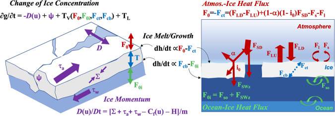
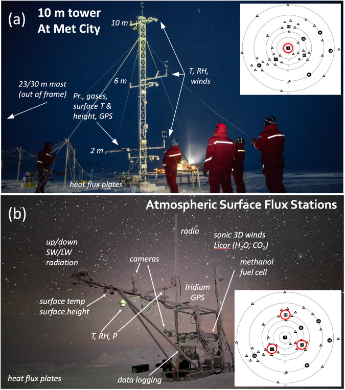
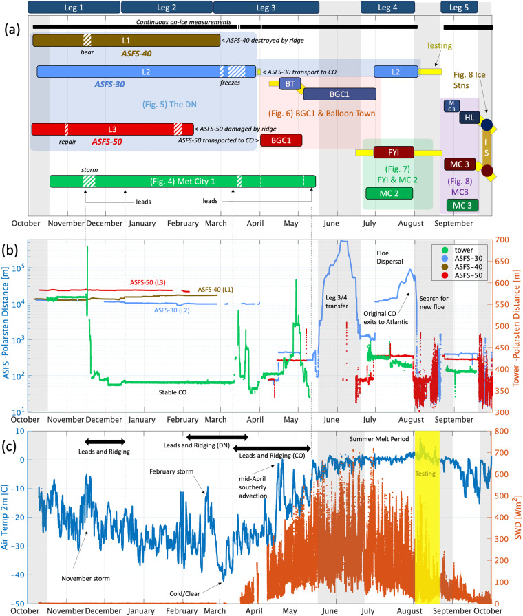
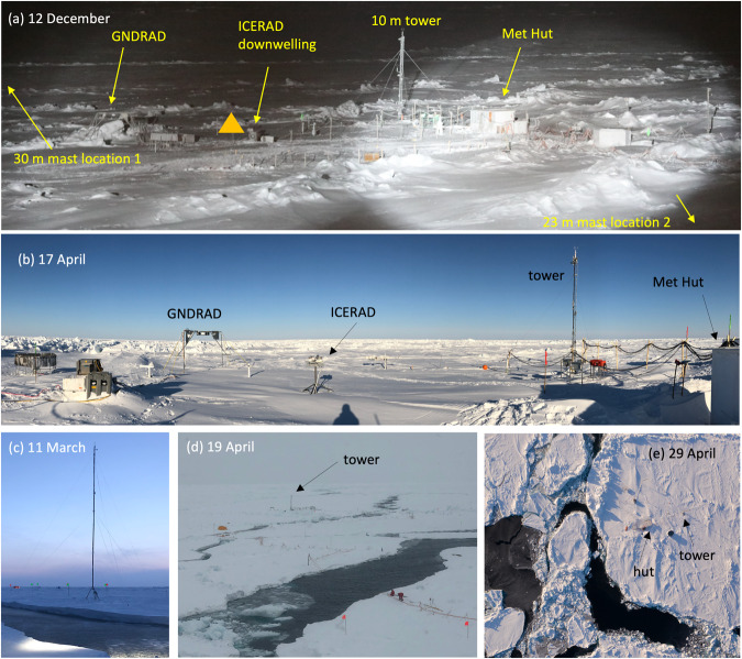
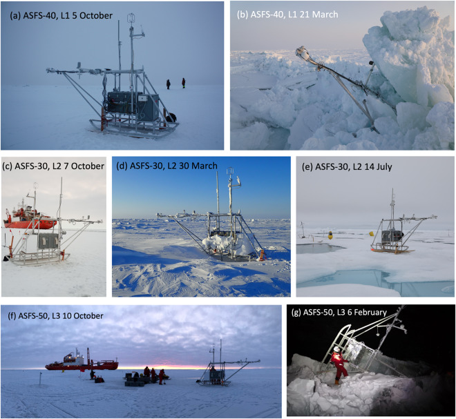
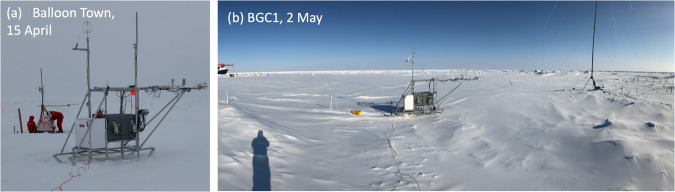
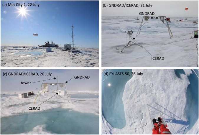
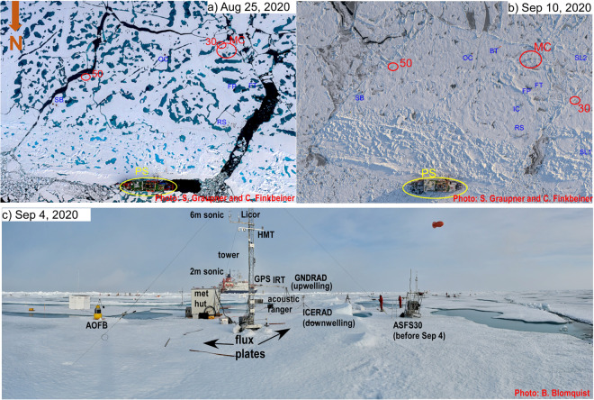
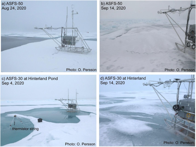
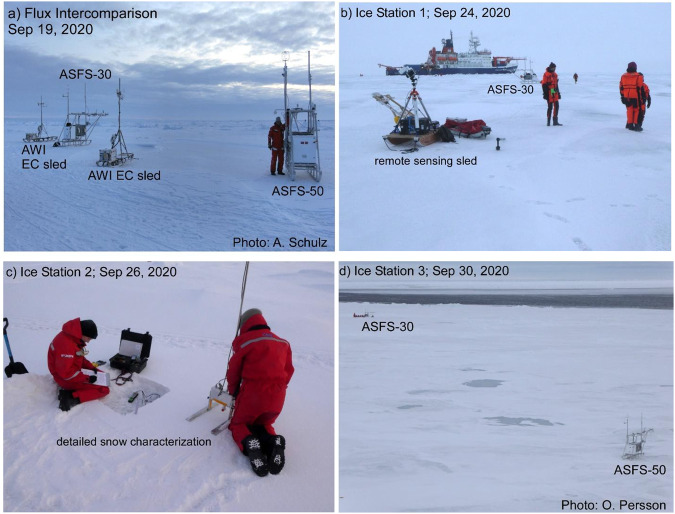
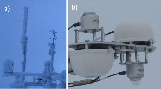
The Multidisciplinary drifting Observatory for the Study of Arctic Climate (MOSAiC) was a yearlong expedition supported by the icebreaker R/V Polarstern, following the Transpolar Drift from October 2019 to October 2020. The campaign documented an annual cycle of physical, biological, and chemical processes impacting the atmosphere-ice-ocean system. Of central importance were measurements of the thermodynamic and dynamic evolution of the sea ice. A multi-agency international team led by the University of Colorado/CIRES and NOAA-PSL observed meteorology and surface-atmosphere energy exchanges, including radiation; turbulent momentum flux; turbulent latent and sensible heat flux; and snow conductive flux. There were four stations on the ice, a 10 m micrometeorological tower paired with a 23/30 m mast and radiation station and three autonomous Atmospheric Surface Flux Stations. Collectively, the four stations acquired ~928 days of data. This manuscript documents the acquisition and post-processing of those measurements and provides a guide for researchers to access and use the data products.

Fig. 1

Schematic and equations of energy transfers affecting sea ice. Dynamic terms are in purple; thermodynamic terms at the surface-atmosphere interface in red (the subject of the present data set), through the ice in blue, and in the ocean in green. D = ice divergence; ψ is mechanical ice redistribution function (ridging); T is thermodynamic ice growth/melt rate; L is lateral melt; u is horizontal ice velocity; τ_a is wind stress; τ_w is ocean stress; Σ is force due to ice interaction; C_f is Coriolis force; H is gravitational acceleration down ocean surface slope; F₀ is net atmosphere-ice heat flux, F_s is atmosphere sensible heat flux; F_l is latent heat flux; F_LD is incoming longwave (LW) flux; F_LU is outgoing LW flux; F_SD is incoming shortwave (SW) flux; α is the surface albedo; i₀ = fraction of absorbed shortwave flux that penetrates into the ice; F_0i = net ocean-ice heat flux; F_so = ocean turbulent sensible heat flux; F_SWz is shortwave radiation reaching ice bottom; F_cb, F_ct are the conductive heat fluxes at ice top and bottom, respectively; dh/dt = melt or growth of ice thickness.

Fig. 2

(a) Image of the tower at Met City in October 2019 (photo by Esther Horvath). (b) Image of ASFS-50 on 1 January 2020 (photo by Michael Gallagher). Both panels are annotated with instrument locations. The insets are maps from the DN at the beginning of Leg 1 with distances in km from Polarstern (large circles) (credit: Daniel Watkins). The red circles in (a) are the CO where the tower was positioned; the three red circles in (b) are the L-sites (L1 lower-left (ASFS-40), L2 (ASFS-30) lower-right, L3 (ASFS-50) top) where ASFS were deployed in October 2019.

Fig. 3

(a) Timeline of installations. “Legs” shown along the top refer to the five legs of the expedition; for precise dates, refer to ref. . Hatch patterns are missing or intermittent data. The vertical grey bars are periods when Polarstern was underway. The horizontal yellow bars are periods of testing and have data of limited scientific use. The black horizontal bar denotes the periods when data were continuous in the aggregate. In (a), the Figures in parentheses illustrate the setup during these time periods, which are described individually under section Observation context and user of assets. MC is a shorted form of “Met City” and the numbers 2 and 3 denote the second and third deployments of Met City, which were at different locations than the original (see main text). (b) Distances between Polarstern and each ASFS (left axis, log scale) and the tower (right axis, linear scale). (c) Composite (tower/all ASFS) temperature (left axis) and shortwave downwelling radiation (F_SD, right axis). The vertical yellow bar marks when Polarstern was underway in search of a new floe and no scientific data were collected from the ice. The data shown during this period is from testing of ASFS-50 carried out on the aft deck of Polarstern: they are not considered scientifically valid and are only shown here for reference.

Fig. 4

Photos of installations associated with Met City 1 (15 October 2019 – 10 May 2020). (a) Original configuration during Leg I after the November storm lead and ridging during which the 30-m mast fell, was rebuilt as 23-m mast, and moved from location 1 to location 2. The orange triangle denotes the approximate position of GNDRAD after it was moved on 17 March. Locations of other installations at Met City are listed for reference. (b) Configuration after GNDRAD and ICERAD were moved on 17 March. (c) 23-m mast at location 2. (d,e) Lead activity between Polarstern and Met City. Photo credit for (e) is ©UFA Show&Factual (unpublished, used with permission).

Fig. 5

Photos of ASFS in the DN. (a) ASFS-40 at L1 on day of deployment, 5 October. (b) ASFS-40 at L1 as it was discovered after ridging events of late Feb/early March. (c) ASFS-30 at L2 on day of deployment, 7 October, Akademik Fedorov in the background. (d) ASFS-30 at L2 on 30 March before being removed to the CO and (e) on 14 July after it was moved back to L2 after being stationed in the CO from April-June. (f) ASFS-50 at L3 on day of deployment, 10 October, Akademik Fedorov in the background. (g) ASFS-50 at L3 as it was discovered after ridging events of early February.

Fig. 6

Photos of ASFS at the CO during Leg 3. (a) ASFS-30 at Balloon Town on 15 April. The AWI mobile flux sled is in the background. (b) ASFS-50 at BGC1 on 2 May. The mast in its third location (13 April – 2 May) is in the background. SIMBA #2020T79 is visible to the left of ASFS-50 in the photo. Note that ASFS-30 was moved into the same position as ASFS-50 in (b), replacing it, on 7 May.

Fig. 7

Met City 2 during Leg 4. (a) Tower and nearby installations at Met City 2 on 22 July. (b,c) ARM ICERAD/GNDRAD systems during period of expansion of melt ponds. (d) Wide-angle photograph of the surface beneath the ASFS-50 boom at First Year Ice (FYI) on 26 July.

Fig. 8

Central observatory floe on (a) 25 August and (b) 10 September 2020. (c) shows Met City 3 instrument installations. The relative locations of Met City 3, ASFS-30 and ASFS-50 are shown in red in (a,b), whereas other installations from other teams are shown in blue (SB-submersible; OC-Ocean City; BT-Balloon Town; FT-Fibertown; FP- flux pond; IC – ice coring; RS – remote sensing; SL1, SL2 – AWI EC sleds). The distance between the Polarstern (yellow oval) and Met City 3 is ~400 m. Photo credit for (a,b) is ©UFA Show&Factual (unpublished, used with permission).

Fig. 9

Photos of ASFS at the CO during Leg 5. (a,b) ASFS-50 at its location near an active and freezing lead for all of Leg 5; (b) ASFS-30 at its location near the met tower from 24 August - 4 September, and (c,d) ASFS-30 at its Hinterland location in a melt pond from 4-19 September, capturing freeze-up.

Fig. 10

Special measurement periods with the ASFS at the end of Leg 5. (a) A turbulent flux intercomparison period was conducted on 19 September between the ASFS and the AWI flux sleds. (b,c,d) three ice stations were conducted during the return transit using ASFS along transects to measure the spatial variability of the energy fluxes and obtain independent estimates of emissivity. These were done in conjunction with measurements by the cryospheric and remote sensing teams along identified transects.

Fig. 11

(a) Photo of sonic anemometer at L2 on 26 October 2019 during icing conditions being managed on 8 W of heating. (b) ASFS-50 3 September 2020 0520 UTC. Rare events of icing on Hukseflux pyranometers occurred on a few days in late August and early September 2020, generally due to freezing fog. These were cleaned on a daily basis.

Fig. 12

(a) Cospectra based on the mean of all sequential 10-minute integration periods from the 10 m tower sensor on two days, 3 and 8 December, 2019, when F_s was predominantly positive (cyan/blue) and negative (yellow/red). Cyan and yellow are data prior to the correction while blue and red are after; at frequencies where only the latter is visible, the spectra are identical. Dashed lines are −8/3 reference, here plotted using a linear y-scale. For reference, data from a nearby Metek USA-1 (that did not contain the artefact) that was mounted to the mast is also shown (greens). The mast height was 4 m on 3 December and was raised from 4 m to 18 m on 8 December. The peak being shifted to higher frequencies at the 4 m height is consistent with the sensor being closer to the surface than the 10 m tower sensor. The data after the mast was raised (light green) show the shift toward peaking at lower frequencies, more similar to the 10 m sensor. (b) Coefficient, β, as a function of frequency under well-mixed (windy and isothermal) conditions. Reds are sensors mounted on the tower and blues are ASFS stations. The number of included times ranged per sensor from N = 3627 (ASFS-40) to N = 7055 (10 m tower).

Fig. 13

Scatterplots of σ_w/u_* (in 10 min segments) as a function of tower-relative wind direction for five time periods during the MOSAiC year. The horizontal black dashed line is the expected value of 1.25. For each period, the boxes show the points for airflow from the ship (cyan), the tower (black; 2 m and 6 m only), and the Met Hut (black; all levels) towards the respective sonic anemometers. The points for which the airflow is coming from the ship (cyan) and the distance to the ship is less than the calculated turbulent footprint size (see text) are circled in magenta. Values when airflow is from the ship are often elevated, especially for the 10 m height when the ship distance is less than the footprint size. Values for winds from the tower and the met hut are often elevated, but not as consistently and as significantly as from the ship at 10 m height.

Fig. 14

Impact of editing eddy covariance values when plotted as a function of bulk values for two MOSAiC time periods. Shown are (a,b) u_* and (c,d) F_s. The red points are the ones removed by the editing routines. Also shown are the correlation coefficients before and after editing and the percentage of points removed. The red and blue lines show the best fit to the unedited and edited data points, respectively. The black dashed line is the 1:1 line. See text for further information.

Fig. 15

Estimates of uncertainty in F_SD as a function of solar zenith angles (SZA) representative of the range observed at MOSAiC. Calculations are valid for clear skies. Diffuse fluxes are estimated to have a flat uncertainty of 3 Wm⁻². Calculations are made individually for each SR30 using unique values provided by the manufacturer, temperature response, and directional response. All other values, including all values for the PSP are nominal specifications of the instrument model.

Fig. 16

2-6-10 m temperature gradients relative to the temperature at 2 m height along the tower averaged for three different conditions: stable wintertime conditions (November-February) (blue); summertime (June-July) during the high solar zenith angle time of day (yellow); and low solar zenith angle time of the day (red). The dashed black line is the dry adiabat.

References

1. Stroeve J, Notz D. Changing state of arctic sea ice across all seasons. Environ. Res. Lett. 2018;13:103001. doi: 10.1088/1748-9326/aade56. - DOI
1. Knust R. Polar Research and Supply Vessel POLARSTERN operated by the Alfred-Wegener-Institute. J. Large-scale Res. Facil. 2017;3:1–8. doi: 10.17815/jlsrf-3-163. - DOI
1. Shupe M, et al. Overview of the MOSAiC Expedition: Atmosphere. Elementa: Sci. Anthro. 2022;10:00060. doi: 10.1525/elementa.2021.00060. - DOI
1. Nicolaus, et al. Overview of the MOSAiC expedition: Snow and sea ice. Elementa: Sci. Anthro. 2022;10:000046. doi: 10.1525/elementa.2021.000046. - DOI
1. Rabe, et al. Overview of the MOSAiC expedition: Physical Oceanography. Elementa: Sci. Anthro. 2022;10:00062. doi: 10.1525/elementa.2021.00062. - DOI
Publication types