CAVE: Connectome Annotation Versioning Engine

Abstract

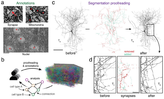
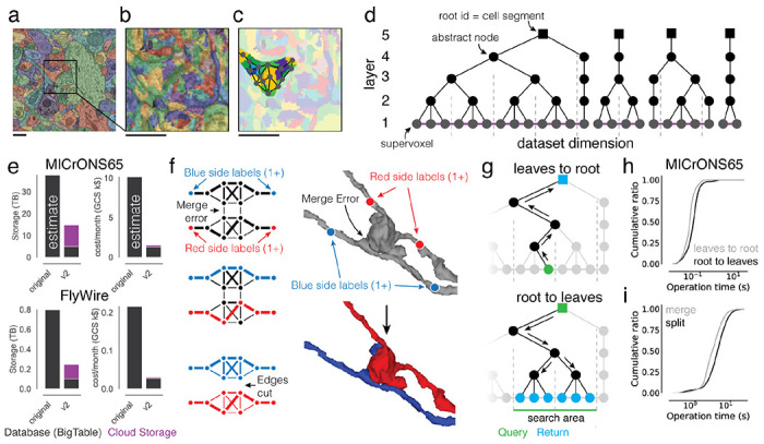
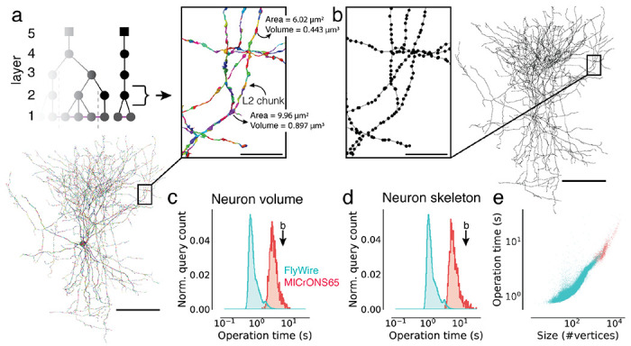
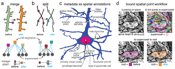
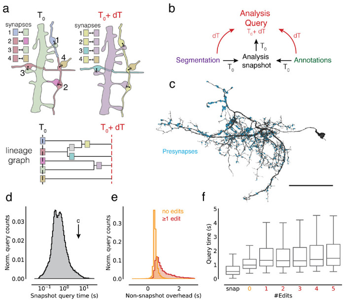
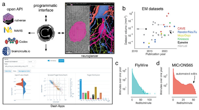
Advances in Electron Microscopy, image segmentation and computational infrastructure have given rise to large-scale and richly annotated connectomic datasets which are increasingly shared across communities. To enable collaboration, users need to be able to concurrently create new annotations and correct errors in the automated segmentation by proofreading. In large datasets, every proofreading edit relabels cell identities of millions of voxels and thousands of annotations like synapses. For analysis, users require immediate and reproducible access to this constantly changing and expanding data landscape. Here, we present the Connectome Annotation Versioning Engine (CAVE), a computational infrastructure for immediate and reproducible connectome analysis in up-to petascale datasets (~1mm³) while proofreading and annotating is ongoing. For segmentation, CAVE provides a distributed proofreading infrastructure for continuous versioning of large reconstructions. Annotations in CAVE are defined by locations such that they can be quickly assigned to the underlying segment which enables fast analysis queries of CAVE's data for arbitrary time points. CAVE supports schematized, extensible annotations, so that researchers can readily design novel annotation types. CAVE is already used for many connectomics datasets, including the largest datasets available to date.

Extended Data Figure 2-1.. Translating user inputs to graph splits.

(a) Bipartite split labels are applied to locations in space. (b) The closest supervoxels to label points are identified (red/blue dots). The supervoxel graph in the neighborhood of the labeled points is computed (graph), weighted by affinity between supervoxels. (c) Vertices along the shortest paths between each pair of red/blue labels are found (black dots and edges). Backup methods prevent overlap between paths. (d) Affinity between vertices along shortest paths is set to infinity and min cut is computed on the path-augmented supervoxel graph.

Extended Data Figure 2-2.. ChunkedGraph performance measurements on FlyWire.

These measurements are from the improved ChunkedGraph implementation using the same FlyWire supervoxel graph that was used for the original implementation. (a) Performance measurement from real-world user interactions measured on the ChunkedGraph server for reads, specifically leaves to root (median=41ms, N=13,410) and root leaves (median=55ms, N=50,001) operations, and (i) edits, specifically merge (median=2,734ms, N=4,189) and split (median=3,486ms, N=2,875) operations.

Extended Data Figure 3-1.. Analysis of timings to calculate morphological features.

Each dot is a query for a single neuron. (a) Times to retrieve a list of L2 chunks for a neuron (root id). (b) Time to look up volume measurements for all L2 chunks belonging to a given neuron. (c) Total time to calculate volumes for neurons.

Extended Data Figure 5-1.. Annotation query timing analysis.

(a) Query times from Fig. 5d versus the size of the query in number of presynapses. (b) Comparing snapshot and non-snapshot aligned presynapse queries for cases where the neuron was not edited between the snapshot and the query time. The difference is the overhead of the mapping logic. The green dashed line is a linear fit with intercept 0.44s and a slope of 1.05.

Figure 1.. Proofreading and analysis of connectomics datasets.

(a) A rich set of ultrastructural features can be extracted from EM images and used for analysis. The corresponding ultrastructural features are annotated with a red *. The synapse is annotated with a red arrow pointing from the pre- to the postsynaptic site. (b) Large connectomics datasets are proofread, annotated, and analyzed by a distributed pool of users in parallel. (c) Proofreading adds and removes fragments from cell fragments (left: before proofreading, center: removed and added fragments, right: after proofreading). (d) Synapse assignments have to be updated with proofreading. All synapses (within the cutout) that were added and removed though the proofreading process of the cell in (c) are shown. Scale bars: 100 μm (c), 1 μm (a: synapse, mitochondria), 10 μm (a: nuclei), 20 μm (d)

Figure 2.. Scaling the ChunkedGraph to petascale datasets.

(a) Automated segmentation overlaid on EM data. Each color represents an individual putative cell. (b) Different colors represent supervoxels that make up putative cells. (c) Supervoxels belonging to a particular neuron, with an overlaid cartoon of its supervoxel graph. This panel corresponds to the framed square in (a) and the full panel in (b). (d) One-dimensional representation of the supervoxel graph. The ChunkedGraph data structure adds an octree structure to the graph to store the connected component information. Each abstract node (black nodes in levels >1) represents the connected component in the spatially underlying graph. (e) Storage and costs for the supervoxel graph storage under the original and the improved implementation (v2). (f) To submit a split operation users place labels for each side of the split (right top). The backend system first connects each set of labels on each side by identifying supervoxels between them in the graph (left). The extended sets are used to identify the edges needed to be cut with a max-flow min-cut algorithm. (g) Examples of graph traversals for looking up the root id for a supervoxel id (top) and supervoxel ids for a root id within a spatially defined search area (bottom). Note that only part of the graph needs to be traversed. (h) Performance measurement from real-world user interactions measured on the ChunkedGraph server for different types of reads and (i) edits. Scale bar: 500 nm

Figure 3.. Fast calculation of morphological features and skeletons.

(a) The basket cell from Fig. 1c broken into L2 chunks where each chunk is colored differently. For each chunk, the L2-Cache stores a number of features such as area, volume, and representative coordinate. (b) A skeleton derived from the ChunkedGraph and L2-Cache without consulting the segmentation data. (c) Client-side timings for calculating neuron volumes using the ChunkedGraph and the L2-Cache for neurons in FlyWire and MICrONS65. The timing for the neuron in (b) is highlighted. (d) Client-side timings for creating skeletons from the ChunkedGraph and the L2-Cache. (e) Client-side timings for creating skeletons plotted against the size of the skeletons. Each dot is a query for a single neuron. Scale bars: 100 μm, insets: 5 μm

Figure 4.. Annotations for proofreadable datasets.

Basic operations of proofreading: (a) merging two objects and (b) splitting two objects. Each edit creates one or more new root objects (cell segments) that represent connected components of the supervoxel graph (octree levels not shown). The changes are tracked in a lineage graph of the altered roots. (c) Spatial points can be used to capture a huge diversity of biological metadata generated by either human annotators or machine algorithms. In CAVE annotations can be created as reference annotations which add additional metadata to existing locations (illustrated as dashed lines). (d) The annotation services handle all annotations through a generic workflow that depends only on expressing all annotations as collections of spatial points and associated metadata. (i) Spatial annotations mark the location of a feature such as a spine head. (ii) The materialization service retrieves the supervoxel id underlying all spatial points. (iii) This enables the materialization service to lookup the root id underneath that points at any given moment in time using the ChunkedGraph.

Figure 5.. Querying the dataset for any time point.

(a) Edits change the assignment of synapses to segment IDs. The lineage graph shows the valid IDs (colors) for each point in time. (b) Analysis queries are not necessarily aligned to exported snapshots. Queries for other time points are supported by on-the-fly delta updates from both the annotations and segmentation through the use of the lineage graph. (c) A neuron in FlyWire with all its automatically detected presynapses. (d) Time measurements for snapshot aligned queries of presynapses for one proofread neuron in FlyWire. (e) The difference between the snapshot and non-snapshot aligned presynapse queries. The two distributions differentiate cases without any edits to the queried neurons and cases with at least one edit to the queried neuron. (f) Presynapse query times for snapshot and non-snapshot aligned queries including cases where neurons were proofread with multiple edits. Scale bar: 50 μm

Figure 6.. Integration into connectomics projects.

(a) CAVE supports multiple interfaces. Besides through programmatic access, users can explore and edit the data in CAVE interactively through neuroglancer or CAVE’S Dash Apps. CAVE integrates with existing and new tools for connectomics though such as natverse, Codex, and braincircuit.io. (b) Datasets published since 2010 by volume and year (volume is plotted on a log-scale). Datasets that were published with manual and semi-automated means are connected with a horizontal gray line. (c) Proofreading rate in edits/min for FlyWire and (d) MICrONS65 over one year of proofreading.

References

1. Briggman K. L. & Bock D. D. Volume electron microscopy for neuronal circuit reconstruction. Curr. Opin. Neurobiol. 22, 154–161 (2012). - PubMed
1. Lichtman J. W. & Denk W. The big and the small: challenges of imaging the brain’s circuits. Science 334, 618–623 (2011). - PubMed
1. Schubert P. J. et al. SyConn2: dense synaptic connectivity inference for volume electron microscopy. Nat. Methods (2022) doi: 10.1038/s41592-022-01624-x. - DOI - PMC - PubMed
1. Dorkenwald S. et al. Automated synaptic connectivity inference for volume electron microscopy. Nat. Methods 14, 435–442 (2017). - PubMed
1. Haberl M. G. et al. CDeep3M-Plug-and-Play cloud-based deep learning for image segmentation. Nat. Methods 15, 677–680 (2018). - PMC - PubMed
Publication types