STENCIL-NET for equation-free forecasting from data

Abstract

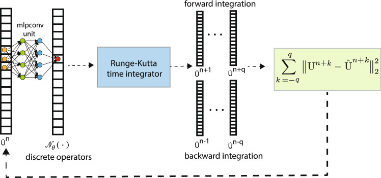
We present an artificial neural network architecture, termed STENCIL-NET, for equation-free forecasting of spatiotemporal dynamics from data. STENCIL-NET works by learning a discrete propagator that is able to reproduce the spatiotemporal dynamics of the training data. This data-driven propagator can then be used to forecast or extrapolate dynamics without needing to know a governing equation. STENCIL-NET does not learn a governing equation, nor an approximation to the data themselves. It instead learns a discrete propagator that reproduces the data. It therefore generalizes well to different dynamics and different grid resolutions. By analogy with classic numerical methods, we show that the discrete forecasting operators learned by STENCIL-NET are numerically stable and accurate for data represented on regular Cartesian grids. A once-trained STENCIL-NET model can be used for equation-free forecasting on larger spatial domains and for longer times than it was trained for, as an autonomous predictor of chaotic dynamics, as a coarse-graining method, and as a data-adaptive de-noising method, as we illustrate in numerical experiments. In all tests, STENCIL-NET generalizes better and is computationally more efficient, both in training and inference, than neural network architectures based on local (CNN) or global (FNO) nonlinear convolutions.

Figure 1

The STENCIL-NET architecture for equation-free forecasting from data. The mlpconv unit performs parametric pooling by moving a small (stencil size $S_m$) MLP network across the input vector ${\widehat{\mathbf{u}}}^n$ at time n to generate the feature maps. The features reaching the output layer are the stencil weights of the discrete propagator ${\mathcal{N}}_{\theta }$. A Runge-Kutta time integrator is used to evolve the network output over time for q steps forward and backward in time, which is then used to compute the loss.

Figure 2

Approximation properties for sharply varying functions. Best rational, polynomial, and MLP fits to the spike function $f(x)=(a+a|x-b|/(x-b))(1/{(x+c)}^2)$ with $a=0.5$, $b=0.25$, and $c=0.1$. The rational function fit uses Newman polynomials to approximate $|x|$.

Figure 3

Numerical solutions of advection of a sharp pulse (red dashed line) using different discretization schemes. (A) Data-adaptive fifth-order WENO stencils; (B) second- and fourth-order central finite differences; (C) first- and third-order upwinding schemes; (D) STENCIL-NET on a $4\times$ coarser grid compared with fifth-order WENO on the same grid. In all plots the advection velocity is $c=2$ in the one-dimensional advection equation $u_t+c{u}_x=0$. All plots are at time $t=3$.

Figure 4

Illustration of data-adaptive stencils. Schematic of the stencil $S_3(x_i)$ centered around the point $x_i$. Here, $S_3(x_i)=S_3^{+}\cup S_3^{-}$.

Figure 5

Comparison between STENCIL-NET (4-fold coarsened) and fifth-order WENO for forced Burgers. (A) Comparison between the STENCIL-NET prediction and WENO data over the entire domain at time $t=40$, i.e., at the end of the training time horizon. (B) Comparison of the nonlinear discrete operators learned by STENCIL-NET (${\mathcal{N}}_{\theta }$) and the ground-truth WENO scheme (${\mathcal{N}}_d$) at time $t=40$.

Figure 6

Forced Burgers forecasting with STENCIL-NET on coarser grids. (A) Left: fifth-order WENO ground-truth (GT) data with spatial resolution $N_x=256$. Right: power spectra of the predictions from different architectures (STENCIL-NET, CNN, FNO) compared to ground-truth. (B,C,D) Left column: output of STENCIL-NET on $2\times$, $4\times$, and $8\times$ coarser grids. The dashed boxes contain the data used for training at each resolution. Right column: point-wise absolute error of the STENCIL-NET prediction compared to the ground-truth (GT) data in (A) beyond the training domain.

Figure 7

STENCIL-NET extrapolation to larger spatial domains and longer times. (A) STENCIL-NET prediction on a $4\times$ coarser grid. (B) Comparison between ground-truth discrete propagator ${\mathcal{N}}_d$ (solid) and STENCIL-NET layer output ${\mathcal{N}}_{\theta }$ (dashed) at times 21 (within training data) and 150 (past training data) marked by dashed vertical lines in (A). The STENCIL-NET was trained on the data within the domain marked by the solid rectangle in (A).

Figure 8

STENCIL-NET generalization to different forcing terms without re-training. Each panel (A,B,C) corresponds to forced Burgers dynamics with a different forcing term (see Eq. 17). Every second row in each panel correspond to point-wise error associated with STENCIL-NET, CNN and FNO (left to right). STENCIL-NET was trained only once using data from (A) (training domain marked by dashed box). Nevertheless, it was able to accurately predict the qualitatively different dynamics for the other forcing terms, since it learned a discrete propagator of the dynamics rather than the solution values themselves. The plots in the first column show the ground-truth data for the different forcing terms, obtained by a fifth-order WENO scheme. The three subsequent columns show the predictions on $4\times$ coarser grids without additional (re-)training and the corresponding absolute errors (w.r.t. WENO) below each plot. The three columns compare STENCIL-NET with a CNN and a FNO of comparable complexity (see Table 1).

Figure 9

Architecture choice, choice of ${\mathit{\lambda }}_{\mathit{wd}}$, and generalization power. All models are trained on the spatio-temporal data contained in the dashed box in Fig. 6. The training box encompasses the entire spatial domain of length $L=2\pi$ and a time duration of $T=40$. (A) STENCIL-NET prediction accuracy (measured as mean squared error, MSE, w.r.t. ground truth) for different network architectures. Only hidden layers are counted, not the input and output layers. Each data point corresponds to the average MSE accumulated over all stable seed configurations. (B) Effect of the weights regularization parameter ${\lambda }_{\mathit{wd}}$ (see Eq. (10) on the prediction accuracy for different training time horizons q. The plots in B were produced with a 3-layer, 64-nodes network architecture, which showed the best performance in A and is used also for all other experiments in this paper. (C) Plots to illustrate the generalization power of trained STENCIL-NET to larger domains. Each data point shows the MSE prediction error from the best model run on the grid of the respective resolution (sub-sample factor) for different domain lengths L and final times T. Training was always done on the data for $L=2\pi$ and $T=40$.

Figure 10

Equation-free forecasting of chaotic Kuramoto-Sivashinsky spatio-temporal dynamics. (Top) Spectral solution of the KS equation on a domain of length $L=64$, where the system behaves chaotically. Data within the dashed rectangle are used for training of the STENCIL-NET model. (Middle) STENCIL-NET forecast on a $4\times$ coarser grid for a $4\times$ longer time. (Bottom) Point-wise absolute difference between the ground-truth data in the top row and the STENCIL-NET forecast in the middle row.

Figure 11

Statistical characteristics of the chaotic system. (Left) Comparison of the power spectral density (PSD) of the ground-truth solution and the STENCIL-NET prediction on a $4\times$ coarser grid. (Right) Growth of the distance between nearby trajectories in the STENCIL-NET prediction, characterizing the maximum Lyaponuv exponent (slope of the dashed red line), compared to the ground truth value $\approx 0.084$ .

Figure 12

Autonomous prediction of chaotic spatio-temporal dynamics. STENCIL-NET can run as an autonomous predictor of long-term chaotic dynamics with different initial condition and for longer times that it was trained for (training data in the dashed rectangle in Fig. 10) and on a (here $4\times$) coarser grid.

Figure 13

STENCIL-NET for learning smooth dynamics from noisy data. (A) Korteweg-de Vries data with point-wise data-dependent additive Gaussian noise of $\sigma =0.1$ used for training. (B) STENCIL-NET prediction after training for 10,000 epochs on a $4\times$ coarser grid using data up to time 1.0 (dashed vertical line). (C) Point-wise absolute error between the STENCIL-NET prediction and the noise-free ground-truth KdV dynamics.

References

1. Karnakov, P., Litvinov, S. & Koumoutsakos, P. Optimizing a DIscrete Loss (ODIL) to solve forward and inverse problems for partial differential equations using machine learning tools. arXiv preprint arXiv:2205.04611 (2022).
1. Pilva, P. & Zareei, A. Learning time-dependent PDE solver using message passing graph neural networks. arXiv preprint arXiv:2204.07651 (2022).
1. Pathak J, Hunt B, Girvan M, Lu Z, Ott E. Model-free prediction of large spatiotemporally chaotic systems from data: A reservoir computing approach. Phys. Rev. Lett. 2018;120:024102. doi: 10.1103/PhysRevLett.120.024102. - DOI - PubMed
1. Pathak J, Lu Z, Hunt BR, Girvan M, Ott E. Using machine learning to replicate chaotic attractors and calculate Lyapunov exponents from data. Chaos: Interdiscip. J. Nonlinear Sci. 2017;27:121102. doi: 10.1063/1.5010300. - DOI - PubMed
1. Vlachas, P. R., Byeon, W., Wan, Z. Y., Sapsis, T. P. & Koumoutsakos, P. Data-driven forecasting of high-dimensional chaotic systems with long short-term memory networks. In: Proceedings of the Royal Society A: Mathematical, Physical and Engineering Sciences474, 20170844 (2018). - PMC - PubMed