Phylogenetic inference from single-cell RNA-seq data

Abstract

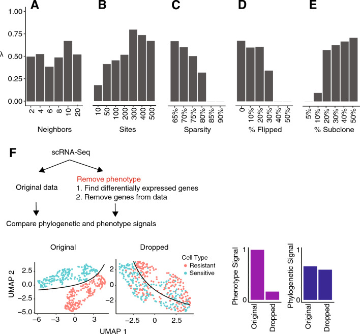
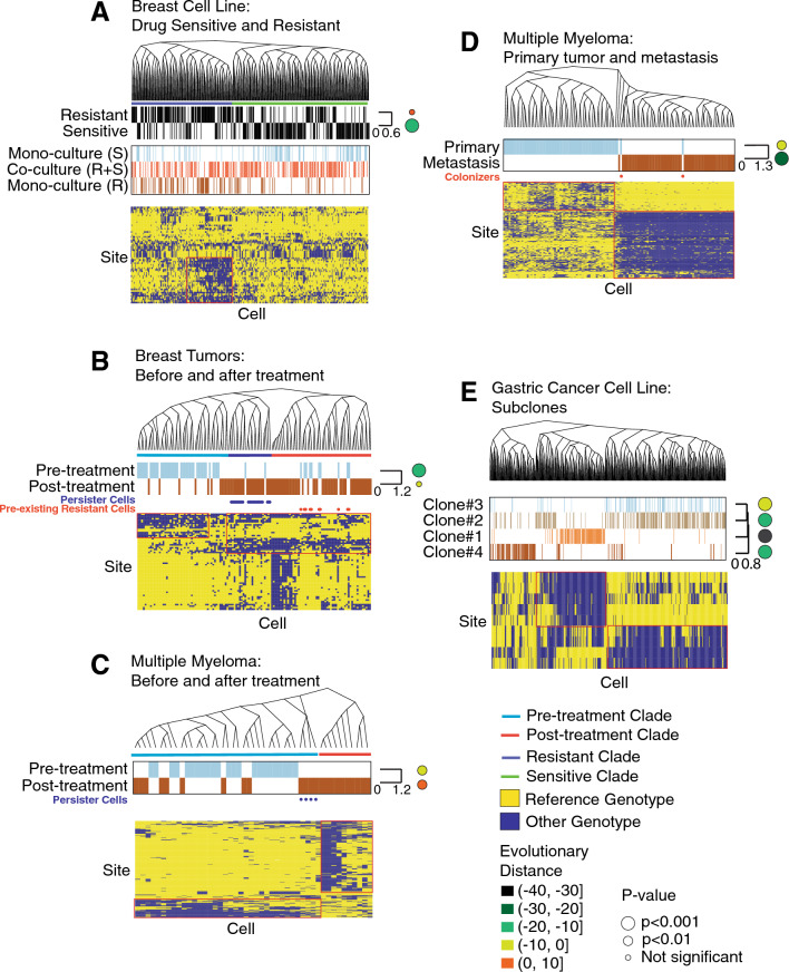
Tumors are comprised of subpopulations of cancer cells that harbor distinct genetic profiles and phenotypes that evolve over time and during treatment. By reconstructing the course of cancer evolution, we can understand the acquisition of the malignant properties that drive tumor progression. Unfortunately, recovering the evolutionary relationships of individual cancer cells linked to their phenotypes remains a difficult challenge. To address this need, we have developed PhylinSic, a method that reconstructs the phylogenetic relationships among cells linked to their gene expression profiles from single cell RNA-sequencing (scRNA-Seq) data. This method calls nucleotide bases using a probabilistic smoothing approach and then estimates a phylogenetic tree using a Bayesian modeling algorithm. We showed that PhylinSic identified evolutionary relationships underpinning drug selection and metastasis and was sensitive enough to identify subclones from genetic drift. We found that breast cancer tumors resistant to chemotherapies harbored multiple genetic lineages that independently acquired high K-Ras and β-catenin, suggesting that therapeutic strategies may need to control multiple lineages to be durable. These results demonstrated that PhylinSic can reconstruct evolution and link the genotypes and phenotypes of cells across monophyletic tumors using scRNA-Seq.

Figure 1

Construction of phylogeny from scRNA-Seq data. (A) Generating a phylogeny from scRNA-Seq alignments consists of three major steps: (1) extracting the read counts, (2) calling and smoothing the genotypes, and (3) reconstructing the phylogeny. (B) The read count extraction process: We start with the alignments of cells from a single-cell RNA-Seq experiment. To extract matrices of read counts, we identify sites of interest by merging the alignments in a pseudobulk sample and calling variants. Then, at each of the variant sites, in each individual cell, we count the number of reads with the reference and alternate alleles. (C) The genotype calling and smoothing processes: We start from matrices of read counts of reference and alternate alleles seen across sites (rows) in single cells (columns). (i) Given the number of reads, we assigned a probability of a (R)eference, (A)lternate, or (H)eterozygous genotype by integrating over a beta-binomial density function. (ii) To compare the genotypes of two cells, we sample 100 genotype profiles by drawing from their probability distributions. (iii) Comparing every pair of cells leads to a pairwise similarity matrix of genetic distance scores. By looking for the highest scores (excluding itself), we find the K nearest neighbors for each cell. (iv) With the nearest neighbors, we can smooth the genotype probability of a cell by averaging with the weighted ($\delta$) average probabilities of its neighbors. We call the genotype with the highest probability score. (D) Phylogenetic reconstruction: We use BEAST2 to infer the phylogeny and produce a final tree using the max clade credibility method.

Figure 2

Smoothing improves the distinction of the genotype profile of the resistant and sensitive cells. (A) Heatmaps show the genotype profile of the resistant and sensitive cells (columns) for the 20 sites (rows) that are most significantly associated with resistance. The heatmaps on the left show the genotype profiles before smoothing, and the ones on the right show the genotype profiles after smoothing. The genotypes are called as either Reference (blue), Alternate (red), or Heterozygous (yellow). Missing data (drop-out) are shown in white. (B) (left panel) The pie chart shows the distribution of the number of reads seen in each element in the site x cell matrix. The fraction of elements with no reads (dropout—the site is not seen in a cell) is shown in grey, the ones with a single read is shown in red, 2–4 reads is green, and at least 5 reads in blue. (middle panel) The tables show how the genotype frequencies changed after smoothing. The elements are discretized into Low (1 read; left table), Medium (2–4 reads; middle table), and High (5+ reads; right table) coverage groups. The columns indicate whether the genotype was Alt(ernate), Het(erozygous), or (Ref)erence before smoothing, and the rows indicate the genotype after smoothing. Each cell in the table indicates the percent of elements that were changed. Each column adds up to 100% (after accounting for rounding artifacts). The Het column in the Low coverage coverage group contains N/A because we cannot call a heterozygous genotype from only 1 read without smoothing. (right panel) The bar plot shows the percent of elements in each coverage group that are changed. (C) The scatter plots show the association between the mean coverage (x-axis) of each mutation site (points) and the correlation of its predicted genotype with the resistance phenotype (y-axis) either before (left plot) or after smoothing (right). Sites associated with the resistance phenotype at p < 0.01 are shown in red.

Figure 3

Impact of data quality and parameters on phylogeny. These barplots show the relationship between the phylogenetic signal λ and (A) number of neighbors, (B) number of sites, (C) sparsity, (D) percent of genotype flipped, and (E) subclone size as percent of all cells. (F) The graphic on the top shows the strategy we use to determine whether the phylogenies are confounded by gene expression patterns. The UMAP plots show the resistant and sensitive cells before (left) and after (right) dropping out 1948 genes associated with resistance. The bar plots represent the resistance signal identified from phenotype (left) and genotype (right) before and after dropping out the resistance-associated genes.

Figure 4

Phylogenetic reconstruction recovers previously identified subclonal lineages across a range of cancer settings. We have generated phylogenies from five scRNA-Seq data sets. The evolutionary distance for each sample condition is shown as the circles at the right of the heatmap. The color and size of the circles represent the evolutionary distance and statistical significance. The yellow (Reference) and blue (Other) heatmaps show the genotypes of the sites with phylogenetic signal K > 0.8 across cells in the phylogeny. If no sites achieved this threshold, we showed the 10 sites with highest K. (A) These cells were experimentally evolved from the parental CAMA-1 cell line to ribociclib sensitive (S) and resistant (R) cell lineages which were then grown in monoculture (alone) or mixed and grown in co-culture (R + S mixed in equal proportions). The cells induced to be drug resistant are shown as black lines in the Resistance bar. The genotypes of the sites with high association with the phylogeny are shown in the heatmap at the bottom. (B) This data set consists of tumor cells collected from ER+ breast cancer tumors before and after treatment. The color bars show the time point of each cell. The phylogeny is divided into clades of pre- (blue) and post-treatment (red) genotypes. Persister cells are delineated with dots. (C) This contains tumor cells from a multiple myeloma patient before and after chemotherapy treatment. The phylogeny is divided into clades of pre- (blue) and post-treatment (red) genotypes. Persister cells are indicated with dots. (D) This data set contains cancer cells collected from the primary or metastasis site from a multiple myeloma patient. (E) This data contains cells from the N87 gastric cancer cell line evolving under untreated conditions. Four subclonal lineages were previously reported to coexist.

Figure 5

Associating the genotypes with phenotypes. (A) The phylogeny from the breast tumor data set in Fig. 4B is reproduced here with new annotations. The phylogeny is split into five clades (A–E). The clades associated with high pathway scores are marked with a colored triangle. The siblings of these clades have low pathway scores. The heatmap on the bottom shows the mean-centered ssGSEA scores for the Hallmark pathways significantly associated with the phylogeny based on phylogenetic signal (fdr < 0.05). Each pathway is labeled with colored triangle(s) that indicate the clade(s) with high pathway score. The phylogenetic associated clades are marked by the horizontal bars below the phylogeny. (B) The violin plots show the ssGSEA scores for the five clades. (C) This phylogeny and its clades are annotated similarly to those in figure A, except that gene mutations are associated with the phylogeny, rather than pathway scores. The heatmap on top shows genes with non-synonymous mutations that are correlated with the phylogeny. The bottom heatmap shows the remaining genes that are correlated with the phylogeny (fdr < 0.01).

References

1. Nowell PC. The clonal evolution of tumor cell populations. Science. 1976;194(4260):23–28. - PubMed
1. Greaves M, Maley CC. Clonal evolution in cancer. Nature. 2012;481(7381):306–313. - PMC - PubMed
1. Swanton C. Intratumor heterogeneity: Evolution through space and time. Cancer Res. 2012;72(19):4875–4882. - PMC - PubMed
1. Beca F, Polyak K. Intratumor heterogeneity in breast cancer. Adv. Exp. Med. Biol. 2016;882:169–189. - PubMed
1. Roth A, et al. PyClone: Statistical inference of clonal population structure in cancer. Nat. Methods. 2014;11(4):396–398. - PMC - PubMed
Publication types