Dynamics of cortical contrast adaptation predict perception of signals in noise

Abstract

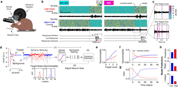
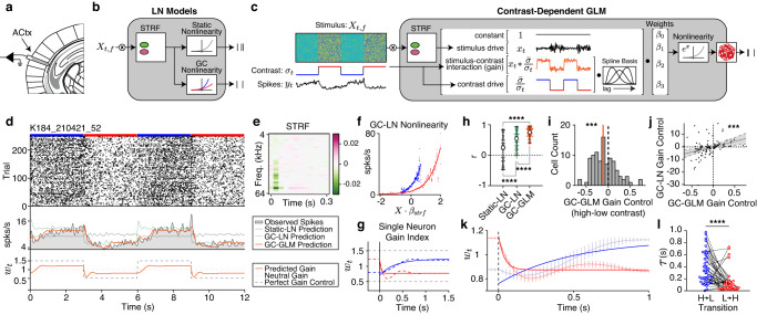
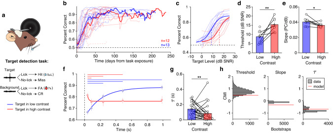
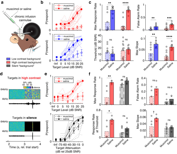
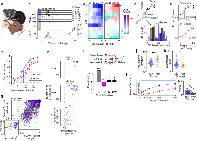
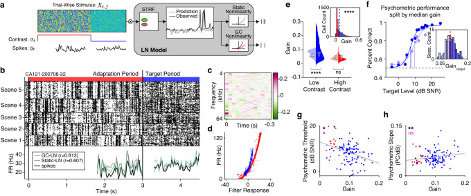
Neurons throughout the sensory pathway adapt their responses depending on the statistical structure of the sensory environment. Contrast gain control is a form of adaptation in the auditory cortex, but it is unclear whether the dynamics of gain control reflect efficient adaptation, and whether they shape behavioral perception. Here, we trained mice to detect a target presented in background noise shortly after a change in the contrast of the background. The observed changes in cortical gain and behavioral detection followed the dynamics of a normative model of efficient contrast gain control; specifically, target detection and sensitivity improved slowly in low contrast, but degraded rapidly in high contrast. Auditory cortex was required for this task, and cortical responses were not only similarly affected by contrast but predicted variability in behavioral performance. Combined, our results demonstrate that dynamic gain adaptation supports efficient coding in auditory cortex and predicts the perception of sounds in noise.

Fig. 1. Target in background detection task and normative model predictions.

a Experimental setup. Tetrode drive images are adapted from ref. . b GO/NO-GO task design. Spectrograms are plotted for example NO-GO and GO trials with transitions from low to high contrast (top row) and high to low contrast (bottom row), with waveforms plotted below each spectrogram (color bar indicates the sound level). Below the example trials, the timing of the response window, schematic licks, and responses to licks are plotted. For NO-GO trials, licks in the response window received a timeout. For GO trials, licks in the response window were rewarded with 5 µL of water. c Example target parameters. Top: varied target levels, with level in dB SNR indicated by the color bar. Bottom: varied target times, where each arrow indicates a potential target delay. d Normative model of efficient gain control. Target and background distributions for each contrast are indicated in the left panel. (1) Target stimuli are indicated with circles, while the background stimulus is indicated by a line. The stimulus response in a given time window is transformed by an adapting nonlinearity to generate spikes. (2) The spiking responses are decoded to update an estimate of the stimulus variance. (3) The gain of the nonlinearity is adjusted to optimally predict the variance of the next timestep. Inset: Example spike distributions of the model neuron in low and high contrast for targets (dark histograms), and background (light histograms). e Model target-from-background discriminability as a function of contrast and target level. Circles indicate model performance overlaid with logistic function fits (solid lines) and thresholds (dashed lines). f Model discriminability over time in low and high contrast. Circles indicate model performance overlaid with exponential function fits. g Model gain dynamics over time in each contrast. h From top to bottom: model predictions for target detection thresholds, slopes, and adaptation time constants in each contrast. Source data are provided as a Source Data file.

Fig. 2. Cortical adaptation to sound contrast is asymmetric.

a Schematic of acute recordings from auditory cortex. Atlas slices were used with permission from figures published in The Mouse Brain in Stereotaxic Coordinates, Third Edition, by Keith Franklin and George Paxinos, pages 49-62, Copyright Elsevier (2007). b Schematic of the linear-nonlinear (LN) model, with a static (gray) or gain-controlled (blue, red) nonlinearity. c A Poisson GLM for estimating gain dynamics. Note that the model estimates gain as the interaction between the stimulus and contrast. Dice graphics were modified by the authors under the Free License based on images from www.vecteezy.com/vector-art/15740075-dice-icon-vector-design-templates. d Top: Spike raster for a representative unit. Blue and red horizontal bars indicate low and high contrast periods of the trial, respectively. Middle: the spike rate of the neuron is overlaid with the predictions from a static LN model, LN model with gain control, or GLM with gain control. Bottom: gain index, $w_t$, estimated from the GLM parameters (Methods). Dashed lines indicate optimal and no gain control (Methods). Orange trace indicates the gain dynamics of the neuron. e Spectro-temporal receptive field (STRF) fit to this neuron. Color bar indicates the strength of the filter response. f Nonlinearities fit to the STRF prediction in low and high contrast. g Dashed blue and red lines indicate the gain index of the example cell in low and high contrast. The overlaid solid lines are exponential fits to the data. h Cross-validated Pearson correlation coefficients between the trial averaged model predictions and spike rates for each model (n = 97 neurons; colors as in d. Error bars indicate 95th percentiles around the median. Asterisks indicate the results of two-way sign-rank tests. i Distribution of gain control estimated by the GLM. Orange line indicates the median. Asterisks indicate the results of a two-way sign-rank test (p = 0.004). j Gain control estimates for each neuron from the GC-GLM and the GC-LN model (black dots) overlaid with the best linear fit (black line) and 95% confidence interval of the fit (gray area). Asterisks indicate whether the linear model was significantly different from a constant model (p = 7.33e−4). k Gain index for all of the neurons with gain control (n = 45). Light lines are the average ±SEM, while the dark lines are exponential fits to the average. l Adaptation time constants from gain-controlled neurons after a switch to low (blue dots) and high contrast (red dots). Asterisks indicate the results of a two-way sign-rank test (p = 6.16e−6). Source data are provided as a Source Data file.

Fig. 3. Target detection performance is consistent with the normative model predictions.

a Schematic of the behavioral setup and task outcomes. Tetrode drive images are adapted from ref. . b Performance as a function of task exposure. Individual traces indicate performance of mice first trained to detect targets in low contrast (blue) or high contrast (red). Thick lines are a 7-day running average across mice in each training group. The dashed red trace near 0.5 was the performance of a mouse who failed to learn the task in high contrast and was excluded from further analysis. c Individual psychometric curves in low and high contrast (n = 12 mice), overlaid with psychometric fits to the average. Dashed vertical lines indicate detection thresholds. d Detection thresholds from the data plotted in c (n = 12 mice; two-way paired t-test: p = 0.0057). e Slopes of the psychometric functions plotted in c (n = 12 mice; two-way paired t-test: p = 0.023). Error bars indicate ±SEM over mice. f Detection performance of threshold level targets presented at different delays from the contrast switch (circles indicate mean ± SEM). Performance is overlaid with exponential fits in each contrast. Horizontal lines above the plot indicate significant sign-rank tests after false-discovery correction. g Adaptation time constants from exponential functions fit to individual mice (n = 21). Asterisks indicate the result of a two-way sign-rank test (p = 0.0060). Error bars indicate ±SEM over mice. h Comparison of average normative model predictions (red lines) to the data (gray distributions) for psychometric thresholds, slopes and adaptation time. The y-axis is the contrast modulation index (CMI, Methods) of the values in each plot. Data distributions were estimated using bootstrapping of the mean (threshold, slope) or median ($\tau$) CMI (10,000 samples with replacement). Source data are provided as a Source Data file.

Fig. 4. Inactivation of auditory cortex selectively disrupts detection of targets in background sounds.

a Schematic of chronic muscimol and saline application in behaving mice. Legend indicates the three potential background conditions in the task. b Behavioral performance on individual sessions (light traces) as a function of contrast (red, blue) and muscimol or saline application (dashed and solid lines, respectively) for n = 44 sessions. -Inf indicates performance on background-only trials. Dots indicate the average performance across sessions ±SEM, overlaid with logistic fits to the data. c Effects of muscimol and contrast on multiple behavioral measures. Bars indicate the mean performance across sessions ±SEM, while dots indicate performance on individual sessions (n = 23 muscimol sessions and 21 saline sessions). Asterisks indicate the significance of two-way rank-sum tests (Supplementary Table 1). d Example spectrograms and waveforms with a target presented in high contrast (top) and the same stimulus when the target was presented in silence (bottom). Color bar indicates the sound level, with black indicating silence. e Behavioral performance in high contrast (top) and in silence (bottom) for n = 26 sessions. Error bars are ±SEM across sessions. Formatting as in b. f The effect of muscimol on multiple behavioral measures when targets were presented in high contrast (red bars; n = 10 sessions) or in silence (black bars; n = 16 sessions). Error bars are ±SEM across sessions. Asterisks indicate the significance of two-way rank-sum tests. Formatting as in c. In all plots: ns not significant; ^†p < 0.1; *p < 0.05; **p < 0.01; ***p < 0.001; ****p < 0.0001. Detailed statistical results for c and f are in Supplementary Table 1. Source data are provided as a Source Data file.

Fig. 5. Cortical responses to targets predict behavioral performance and exhibit contrast adaptation.

a Schematic of chronic recordings during behavior. Tetrode drive images are adapted from ref. . b Spike raster from a neuron recorded during the task with average PSTHs. Inset: area under the ROC curve (AUC) for each level ±bootstrapped 95% CI. c Neurograms of populations of simultaneously recorded neurons in low (left) and high contrast (right) sessions. Color bars indicate the difference in firing rate between the noise-only condition and each target level. The arrow indicates the cell in b. d Upper left: schematic for estimating the population coding direction (CD). Lower right: probability distributions of CD projections for noise-only trials (gray) and the highest-level target trials (blue). The vertical red line indicates the criterion for the decoder. e Neurometric performance and behavioral performance in representative low contrast (top) and high contrast (bottom) sessions. Dark dots are decoder performance, while light dots indicate behavioral performance, overlaid by logistic function fits. The arrow indicates the decoder performance for the distributions in d. f Average psychometric and neurometric performance ±SEM over sessions. Formatting as in e. g Behavioral performance as a function of neurometric performance for n = 102 sessions. Each point is performance at a single target level in a single session. Point color indicates contrast, while point size indicates target level. Dots joined by gray lines were collected in the same session. Inset: Same data as in g, with the effect of target level regressed out (!L). The black line indicates the model fit and 95% CI. h Behavioral performance as a function of neural performance split by target levels. Text indicates the correlation coefficient and its significance value. i Top: the linear model used to predict behavior. Bottom: model coefficients ±standard error for target level (L), contrast (C), neurometric performance (N) terms, and the interaction between the latter two terms (C*N). Asterisks indicate significant predictors (n = 102 sessions). j Neurometric thresholds ±SEM for sessions in low (n = 82) and high contrast (n = 35). Asterisks indicate significant two-way rank-sum test (p = 1.34e−6). k Same as j, but for neurometric slopes (two-way rank-sum test: p = 0.029). l Left: Neurometric performance ±SEM as a function of target delay over sessions (n = 87). Formatting and statistical tests are the same as Fig. 3f. Right: Adaptation time constants ±SEM fit to the neurometric response from n = 12 mice. Asterisk indicates a significant two-way sign-rank test (p = 0.016). Source data are provided as a Source Data file.

Fig. 6. Cortical gain predicts session-to-session variability in behavioral performance.

a Schematic of the LN model fit to neuronal responses during the behavioral task. b Spike raster of a representative unit recorded during the behavioral task, sorted by the background scene presented in each trial. Below is the average spike rate (black trace) overlaid with the LN model fit with a static (gray) or gain-controlled nonlinearity (green). c STRF for the representative cell. d The fitted nonlinearities in low and high contrast periods of the trials. e Gain distributions across all recorded neurons as a function of contrast and trial period (A adaptation, T target). Gain was significantly larger in the target period during low contrast (two-way ANOVA: p = 3.77e−9) but not in high contrast (p = 0.18) Inset: the average gain in low and high contrast for all cells, dashed lines indicate the median of each distribution. Gain was higher in low contrast (two-way ranksum: p = 1.60e−91. f Psychometric curves split by the median gain (n = 107 sessions). Light colored dots indicate performance across sessions with low gain, dark colored dots indicate performance on sessions with high gain. Error bars indicate ±SEM. Inset: the distribution of gain values on the same sessions. The dashed red line indicates the median used to split the data. g Relationship between session-to-session changes in gain and behavioral thresholds (n = 124 sessions). Each dot is a session, with the color indicating the contrast in which targets were presented. The gray line is the linear best fit. Black asterisks indicate whether gain is a significant predictor of the psychometric threshold, while magenta asterisks indicate whether contrast was a significant predictor of behavioral thresholds (Supplementary Table 1). h Same formatting as g, but plotting the relationship between gain and psychometric slope (n = 124 sessions). Source data are provided as a Source Data file.

References

1. Barlow HB. Possible principles underlying the transformations of sensory messages. Sens. Commun. 2013;6:216–234.
1. Brenner N, Bialek W, De Ruyter Van Steveninck R. Adaptive rescaling maximizes information transmission. Neuron. 2000;26:695–702. - PubMed
1. Bharioke A, Chklovskii DB. Automatic adaptation to fast input changes in a time-invariant neural circuit. PLoS Comput. Biol. 2015;11:1004315. - PMC - PubMed
1. Borst A, Theunissen FE. Information theory and neural coding. Nat. Neurosci. 1999;2:947–957. - PubMed
1. Baccus SA, Meister M. Fast and slow contrast adaptation in retinal circuitry. Neuron. 2002;36:909–919. - PubMed
Publication types