Genome-wide prediction of disease variant effects with a deep protein language model

Abstract

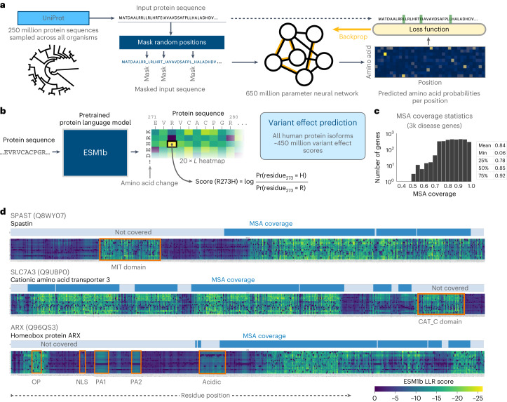
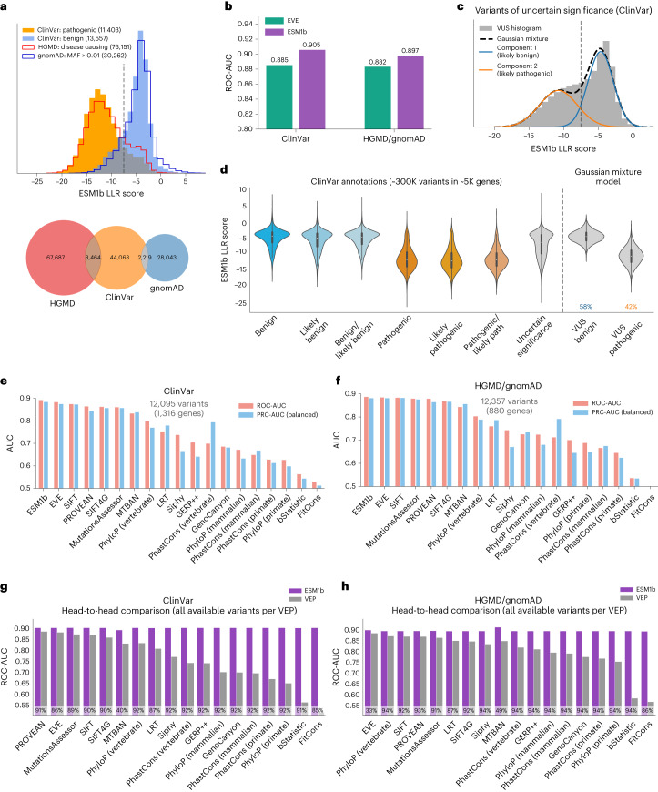
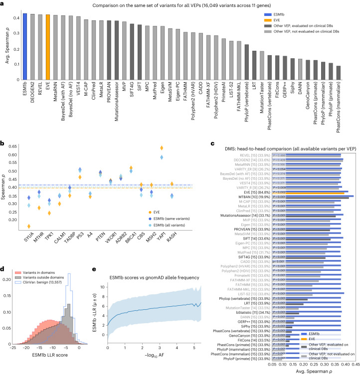
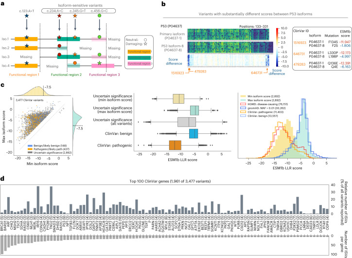
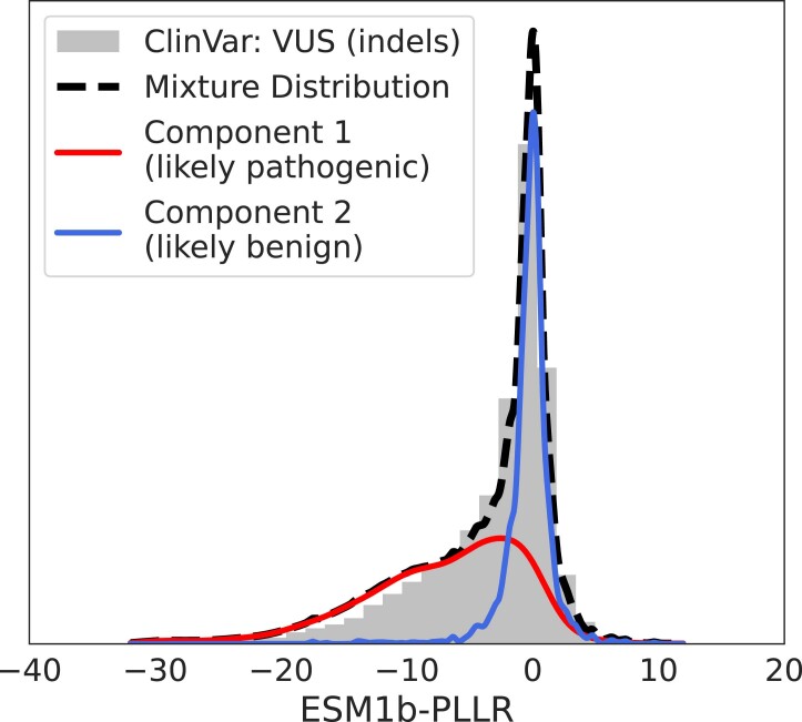
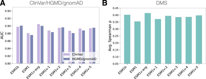
Predicting the effects of coding variants is a major challenge. While recent deep-learning models have improved variant effect prediction accuracy, they cannot analyze all coding variants due to dependency on close homologs or software limitations. Here we developed a workflow using ESM1b, a 650-million-parameter protein language model, to predict all ~450 million possible missense variant effects in the human genome, and made all predictions available on a web portal. ESM1b outperformed existing methods in classifying ~150,000 ClinVar/HGMD missense variants as pathogenic or benign and predicting measurements across 28 deep mutational scan datasets. We further annotated ~2 million variants as damaging only in specific protein isoforms, demonstrating the importance of considering all isoforms when predicting variant effects. Our approach also generalizes to more complex coding variants such as in-frame indels and stop-gains. Together, these results establish protein language models as an effective, accurate and general approach to predicting variant effects.

Fig. 1. ESM1b predicts variant effects without homology coverage.

a, ESM1b is a 650-million-parameter protein language model trained on 250 million protein sequences across all organisms. The model was trained via the masked language modeling task, where random residues are masked from input sequences and the model has to predict the correct amino acid at each position (including the missing residues). b, Illustration of the ESM1b model’s input (an amino acid sequence) and output (LLR of effect scores for all possible missense variants). c, The distribution of MSA coverage (that is, the fraction of a protein’s residues that are aligned) across ~3,000 disease-related proteins covered by EVE. d, Examples of the model’s capacity to detect protein domains and functional regions, including outside MSA coverage, across the following three human proteins: SPAST, SLC7A3 and ARX. Each heatmap visualizes the LLR scores across all 20 × L possible missense variants (where L is the protein length). Protein domains without MSA coverage are highlighted in orange.

Fig. 2. ESM1b is suitable for genome-wide disease prediction of coding variants.

a, Top: the distribution of ESM1b effect scores across two sets of variants that are assumed to be mostly pathogenic (‘ClinVar: pathogenic’ and ‘HGMD: disease causing’) and two sets of variants assumed to be mostly benign (‘ClinVar: benign’ and ‘gnomAD: MAF > 0.01’). Bottom: Venn diagram of the variants extracted from HGMD, ClinVar and gnomAD. b, Comparison between ESM1b and EVE in their capacity to distinguish between pathogenic and benign variants (measured by global ROC-AUC scores), as labeled by ClinVar (36,537 variants in 2,765 unique genes) or HGMD/gnomAD (30,497 variants in 1,991 unique genes). c, The distribution of ESM1b effect scores across ClinVar missense VUS, decomposed as a mixture of two Gaussian distributions capturing variants predicted as more likely pathogenic (orange) or more likely benign (blue). d, The distribution of ESM1b effect scores across all common ClinVar labels, including the two Gaussian components from c. Boxes mark Q1–Q3 of the distributions, with midpoints marking the medians (Q2) and whiskers stretching 1.5× IQR. Altogether there are ~300,000 missense variants labeled in ClinVar. e,f, Evaluation of 19 VEP methods against the same two benchmarks: ClinVar (e) and HGMD/gnomAD (f). Performance was measured by two metrics for binary classification as follows: ROC-AUC (light red) and a balanced version of PRC-AUC (light blue; Methods). Performance was evaluated on the sets of variants available for all 19 methods. g,h, Head-to-head comparison between ESM1b and each of the 18 other VEP methods over the same two dataset benchmarks (in terms of ROC-AUC). Because ESM1b provides scores for all missense mutations, the comparison against each other method is performed on the set of variants with effect predictions for that method. The percentage of variants considered for each method is shown at the bottom of each bar. IQR, interquartile range.

Fig. 3. ESM1b predicts the effects of experimental measurements from DMS.

a, Evaluation of 43 VEP methods (including ESM1b and EVE) on a DMS benchmark containing 28 assays over 15 different human genes (Supplementary Table 1). Of the entire set of 76,133 variants in 15 genes, 16,049 variants in 11 genes obtained effect scores by all 43 VEP methods. We excluded 3 VEP methods, VARITY_ER, VARITY_R and MTBAN (Methods), which would have dramatically reduced the number of variants and genes shared by all methods. The methods are sorted by the average Spearman’s correlation between each method’s scores and the experimental scores. b, The performance of ESM1b and EVE over the 15 individual genes in the DMS benchmark. The average performance of each method is marked by a dashed line. Because ESM1b can process all missense variants (while EVE assigns scores only for a subset of them), the performance of ESM1b is shown either for all variants (‘all variants’) or the subset of variants with EVE scores (‘same variants’). c, Head-to-head comparison between ESM1b and each of the other 45 VEP methods on the DMS benchmark, where each method is compared against the set of variants with predictions for that method. The number of unique genes and percentage of variants with predictions for each method are shown in squared brackets and parentheses, respectively. One-tailed P values indicating significant differences from ESM1b are shown at the beginning (left) of the bars. Methods are sorted by the difference in average Spearman’s correlation between ESM1b and each of the other methods. Comparisons against methods not evaluated on clinical DBs are grayed out. d, The distribution of ESM1b effect scores for variants in annotated protein domains (red) versus variants outside of domains (gray). The distribution of benign variants (as in Fig. 2a) is shown for reference. e, Average ESM1b effect score (and s.d.) as a function of allele frequency over all gnomAD missense variants.

Fig. 4. ESM1b predictions in clinically relevant genes depend on the isoform context.

a, The consequences of variants (for example, damaging versus neutral) can depend on the isoform context. b, Comparison of the primary and one of the alternative isoforms of P53. Three specific variants are detailed. c, Left: all 3,477 ClinVar variants with highly variable ESM1b effect scores across different isoforms (defined by s.d. > 2). Center: the lowest and highest isoform scores predicted for all VUS from the left panel (top two boxes), compared to the mean scores (across isoforms) of VUS, benign or pathogenic variants (as in Fig. 2d; bottom three boxes). The boxes represent the Q1–Q3 range and median (Q2) line; whiskers correspond to 1.5× IQR; outliers (outside the whiskers) are shown individually. Right: the distribution of the lowest and highest isoform scores predicted for all VUS from the left panel, compared to the distributions for pathogenic or benign variants from ClinVar, HGMD and gnomAD (as in Fig. 2a). Across all panels, the number of variants associated with each category is shown in parentheses. d, The top 100 ClinVar genes with the highest number of variants with highly variable effect scores (as in c). Numbers of annotated isoforms of each gene are shown in parentheses.

Fig. 5. ESM1b can detect isoform-specific variant effects.

a, Approximately 1.8 million missense variants across ~9,000 genes in the human genome are ‘isoform sensitive’, defined by (1) maximum ESM1b effect score (across isoforms) > −7, (2) minimum score < −8 and (3) difference between minimum and maximum score > 4. b, Top: ISV are closer to splice junction than would be expected at random. Bottom-left: ISV in genes with domains containing splice junctions: 90.31% versus 28.21% expected at random. Bottom-right: metrics of predicting whether genes contain domains disrupted by splice junction given whether or not they contain ISV. c, An example of a small splicing effect (excision of five amino acids from the primary isoform of the MEN1 protein) leading to dramatic changes in the predicted effects of variants in a much larger region. Bottom: AlphaFold structural predictions of the two isoforms. Arrows are pointing to a small surface pocket introduced by the five amino acid deletion (around Ser145). d, An example of alternative splicing leading to a distant effect in the TGFB3 proprotein. Exclusion of the TGFβ-3 chain in an alternative isoform of the proprotein leads to a region at the beginning of the LAP chain (marked by orange) losing its sensitivity to missense variants. Right: AlphaFold prediction of the binding of the two chains showing these two regions to be close to one another in 3D structure. ISV, isoform-sensitive variants; ACC, accuracy; TPR, true-positive rate; F1, F1 score; MCC, Matthew’s correlation coefficient.

Fig. 6. ESM1b effect predictions generalize to any coding variant.

a, Top: functional effect scores are assigned to in-frame indels by invoking ESM1b on both the WT and mutated protein sequence and calculating the PLLR between them. Bottom: the distribution of ESM1b effect scores over 1,679 benign and 1,791 pathogenic in-frame indels from ClinVar. b, Comparison between three versions of ESM1b-based effect scores, CADD (a supervised VEP method) and three baseline models as classifiers of pathogenic versus benign in-frame indels (over the same set of variants as in a). One-tailed P values are shown for the differences between the performance of CADD and the ESM1b-based effect scores (Methods). Right: partitioning of the 3,470 in-frame indels into deletions, insertions and deletion–insertion combinations (delins). c, Functional effect scores are also assigned to stop-gain variants, defined as the LLR score assigned to the missense variant predicted to be the most deleterious among all possible missense variants in the lost region of the protein. Illustrated example: substitution of a glutamine into a stop codon at position 25. d, Assessment of ESM1b and three baseline models as classifiers of pathogenic versus benign stop-gain variants, over variants expected to either (1) not undergo NMD (3,672 pathogenic and 147 benign variants), (2) undergo NMD (32,362 pathogenic and 198 benign variants) or (3) all stop-gain variants (36,034 pathogenic and 345 benign variants). Error bars correspond to s.d. of the ROC-AUC scores centered around the mean (estimated by bootstrapping).

Extended Data Fig. 1. Comprehensive evaluation of ESM1b and EVE on ClinVar, HGMD/gnomAD and deep mutation scans.

(a) ROC curves of ESM1b and EVE as binary classifiers of variant pathogenicity over ClinVar (left) and HGMD/gnomAD (right). The true positive rate at the standard false positive rate (0.05) is annotated across all 4 curves. (b) Evaluation of EVE (left bar plots) and ESM1b (right bar plots) over ClinVar (top panels) and HGMD/gnomAD (bottom panels), using either the global ROC-AUC (red) or gene-average ROC-AUC (yellow) metric (see the relevant section in the Methods). For each dataset, we show the results for either the full dataset (left panels), or the subsets of variants in long (middle panels) or short (right panels) proteins (defined by a threshold of 1,022aa, which is the maximum window length supported by ESM1b; see Methods). Dashed lines: the top score (obtained by ESM1b or EVE) according to each of the two metrics. (c) Evaluation of ESM1b and EVE on deep mutational scanning datasets over each of the 28 assays (which were aggregated per gene in Fig. 3b).

Extended Data Fig. 2. Per-gene evaluation of top VEP methods on deep mutational scans.

Per-gene DMS results for the 9 VEP methods that are closest to ESM1b in performance according to the head-to-head comparison (Fig. 3c). The numbers of unique variants scored by each VEP method, out of the total 76,133 variants in the full DMS dataset, are shown in square brackets next to the method names. The numbers of variants per gene are shown in parentheses next to the gene names.

Extended Data Fig. 3. Estimating the pathogenicity rate among indel variants of uncertain significance.

In gray: the distribution of ESM1b PLLR effect scores across indels in ClinVar annotated as variants of uncertain significance (VUS). We estimated the fraction of pathogenic and benign variants among these VUS indels by decomposing the VUS distribution of effect scores as a mixture of the distributions over pathogenic and benign variants (Fig. 6a) approximated by kernel density estimation. Red and blue curves: the mixture components of pathogenic and benign effect scores, respectively. Black dashed curve: the sum of the pathogenic (red) and benign (blue) components as an estimate of the empirical distribution of VUS (gray).

Extended Data Fig. 4. Evaluation and comparison of different ESM models.

Tested ESM models: ESM1b, ESM1, the five ESM1v models, and an assembly of the five ESM1v models into a single model averaging the LLR scores obtained by the 5 models (ESM1v-avg). (a) Performance of the different ESM models on the clinical benchmarks (ClinVar and HGMD/gnomAD). Each model was evaluated as a binary classifier of pathogenic vs. benign missense variants over the two benchmarks using the global ROC-AUC metric. Only proteins smaller than 1,022aa were considered in this evaluation (thereby avoiding the sliding window approach). (b) Performance of the ESM models on the DMS benchmark.

Extended Data Fig. 5. The sliding-window approach to tile long protein sequences with ESM1b.

(a) The variant weights over each window’s coordinates (1 ≤ i ≤ 1022), defined by the function: w(i) = 1 / (1 + exp(-(i-128)/16) for 1 ≤ i < 256, w(i) = 1 for 256 ≤ i < 1022-256, and w(i) = 1/(1 + exp((i-1022 + 128)/16) for 1022-256 ≤ i ≤ 1022. (b) An example tiling of a protein sequence of length 1,479aa. Left: raw window weights (as in (a)). Right: normalized weights (summing up to 1 at each protein position). (c) Example of how a specific protein isoform (UniProt ID Q7Z460-5) is tiled. Top panel: ESM1b effect scores over the left window (1 ≤ i ≤ 1022; orange), the right window (458 ≤ i ≤ 1479; green), and the final weighted average throughout the entire protein’s length (blue). Middle: ESM1b effect scores over the left window. Bottom: ESM1b effect scores over the right window. (d) An example tiling of a larger protein sequence of length 3,703aa, as in (b). Top: the locations of the 7 windows used to tile the sequence. Middle: raw window weights. Bottom: normalized weights. (e) Example of how a specific protein (UniProt ID Q15911) is tiled, as in (c). As shown in the two examples, the effect scores tend to be consistent across different windows (with edge effects sometimes being more pronounced).

Extended Data Fig. 6. Evaluation of different sliding window approaches and window sizes.

(a) Evaluation as binary classifiers of variant pathogenicity over the ClinVar dataset (global ROC-AUC metric). (b) Evaluation over short proteins (640 to 900aa), by comparing the scores obtained from processing the entire sequences through a single window vs. multiple windows. Three metrics are considered for comparing the scores: Spearman’s correlation (left), mean square error (center) or 95th percentile of absolute difference (right). Comparison was performed over 500 randomly chosen proteins of length 640 to 900aa. To accommodate different window sizes with the weighted-average approach, we rescaled the range of the sigmoid function (described in Extended Data Fig. 5) in proportion to the window size. Points along the curves correspond to the mean metric values across the 500 proteins; error bars correspond to 95% confidence intervals for the means.

References

1. Brandes N, Weissbrod O, Linial M. Open problems in human trait genetics. Genome Biol. 2022;23:131. doi: 10.1186/s13059-022-02697-9. - DOI - PMC - PubMed
1. Richards S, et al. Standards and guidelines for the interpretation of sequence variants: a joint consensus recommendation of the American College of Medical Genetics and Genomics and the Association for Molecular Pathology. Genet. Med. 2015;17:405–424. doi: 10.1038/gim.2015.30. - DOI - PMC - PubMed
1. Rehm HL, Fowler DM. Keeping up with the genomes: scaling genomic variant interpretation. Genome Med. 2019;12:5. doi: 10.1186/s13073-019-0700-4. - DOI - PMC - PubMed
1. Frazer J, et al. Disease variant prediction with deep generative models of evolutionary data. Nature. 2021;599:91–95. doi: 10.1038/s41586-021-04043-8. - DOI - PubMed
1. Buniello A, et al. The NHGRI-EBI GWAS catalog of published genome-wide association studies, targeted arrays and summary statistics 2019. Nucleic Acids Res. 2018;47:D1005–D1012. doi: 10.1093/nar/gky1120. - DOI - PMC - PubMed
Publication types