Extensive investigation of geometric effects in sonoreactors: Analysis by luminol mapping and comparison with numerical predictions

Abstract

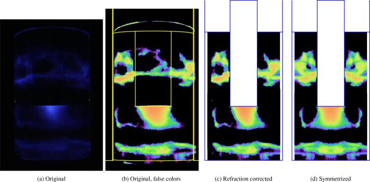
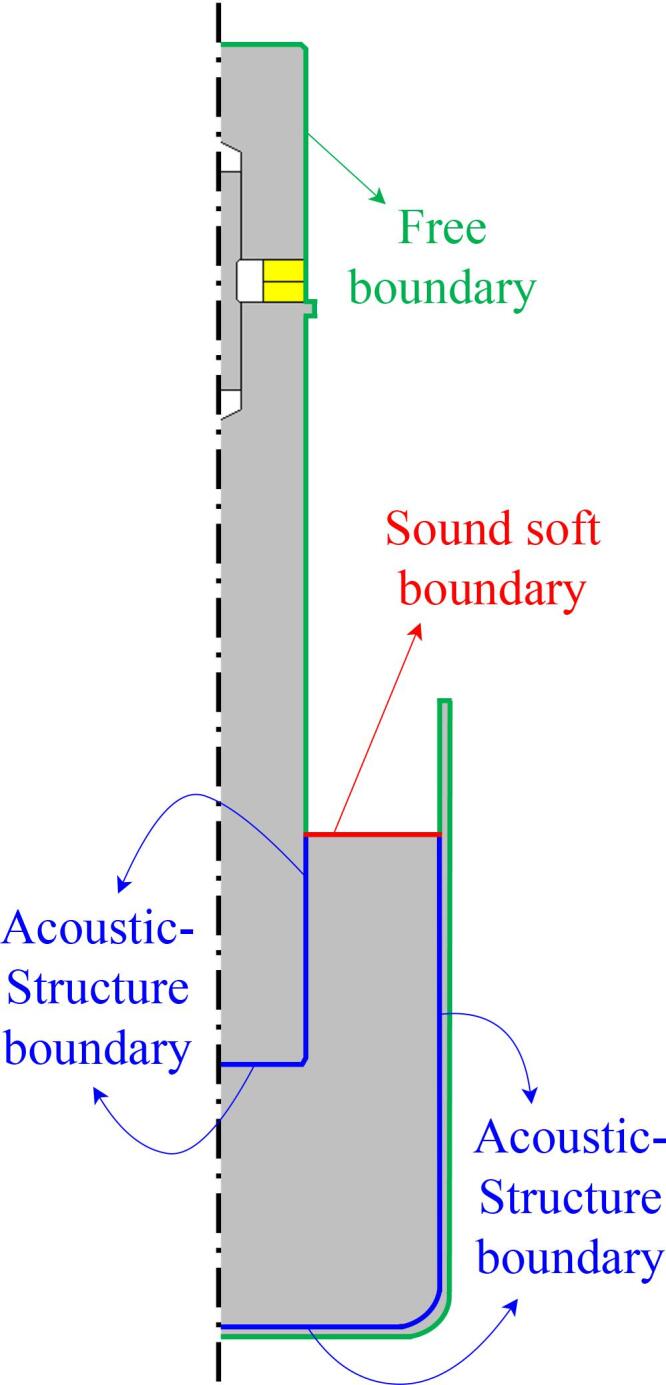
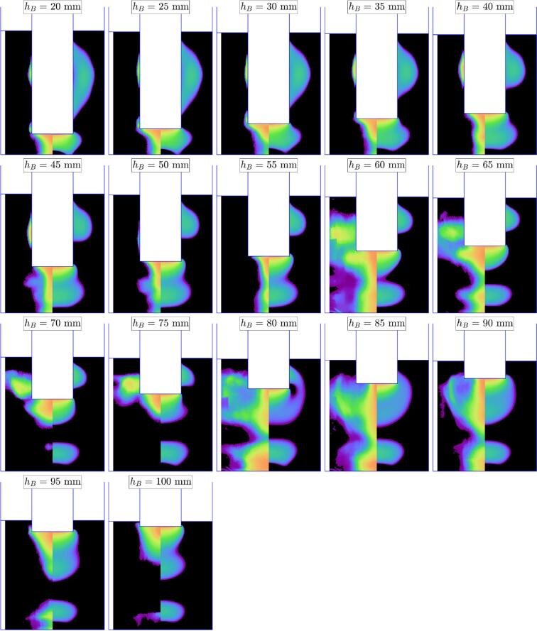
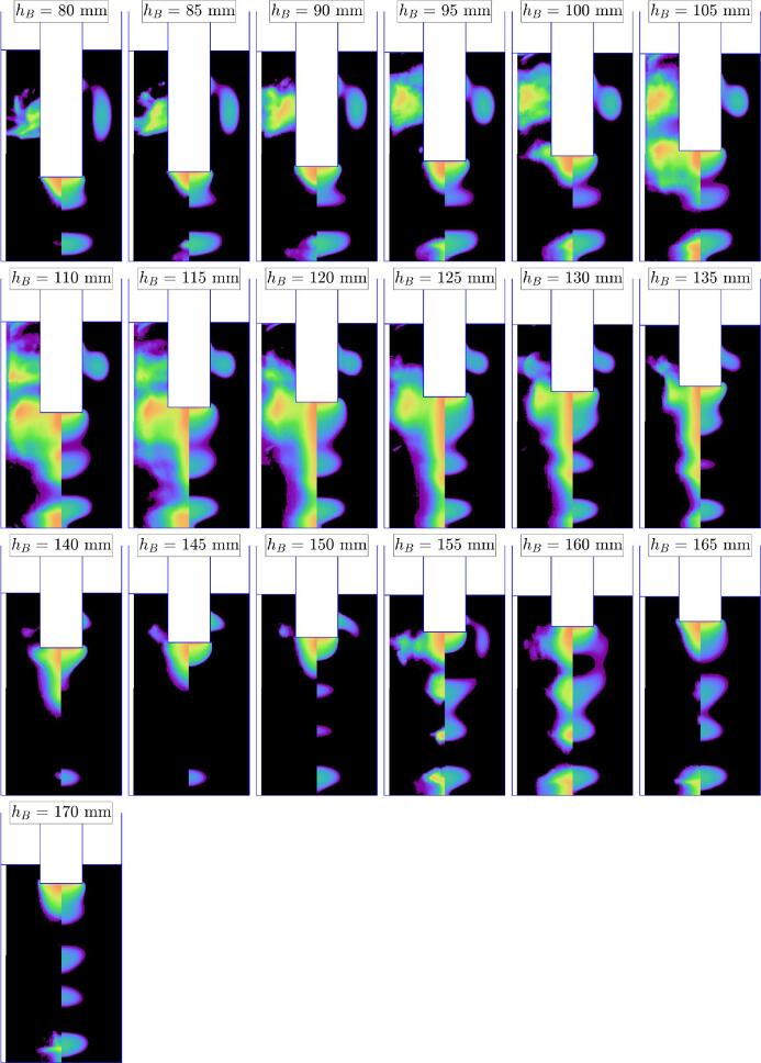
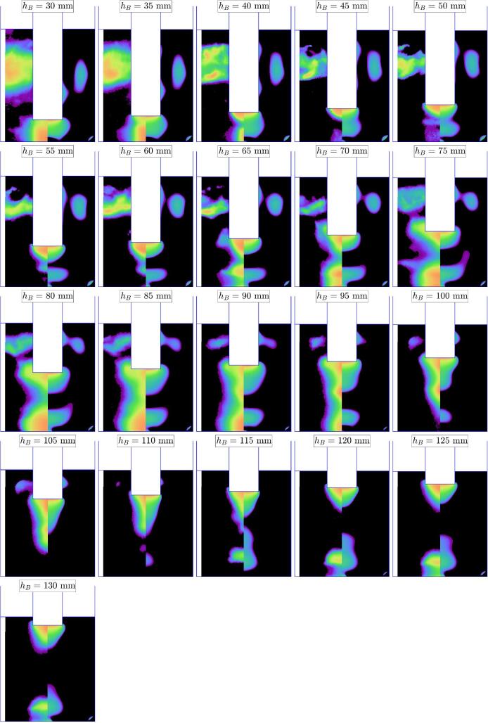
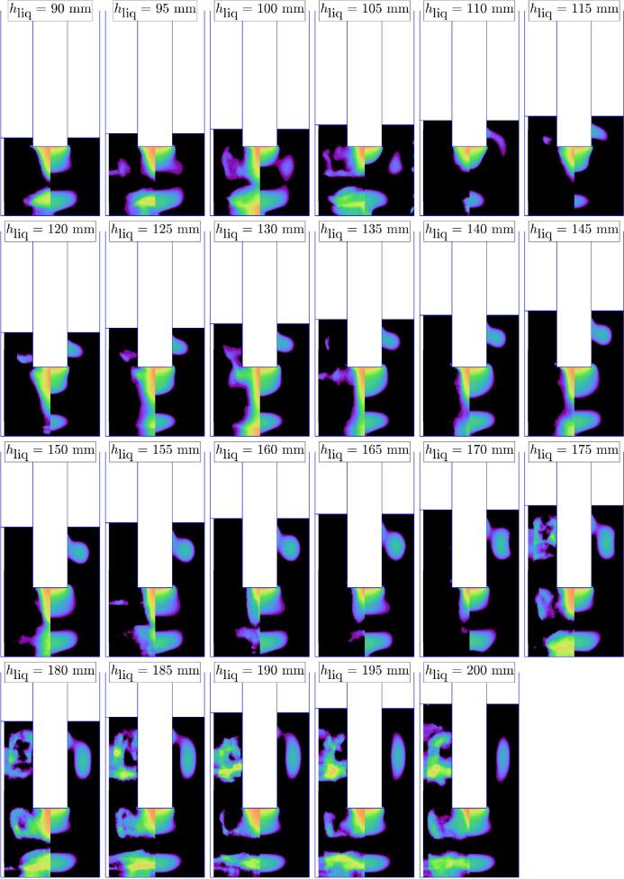
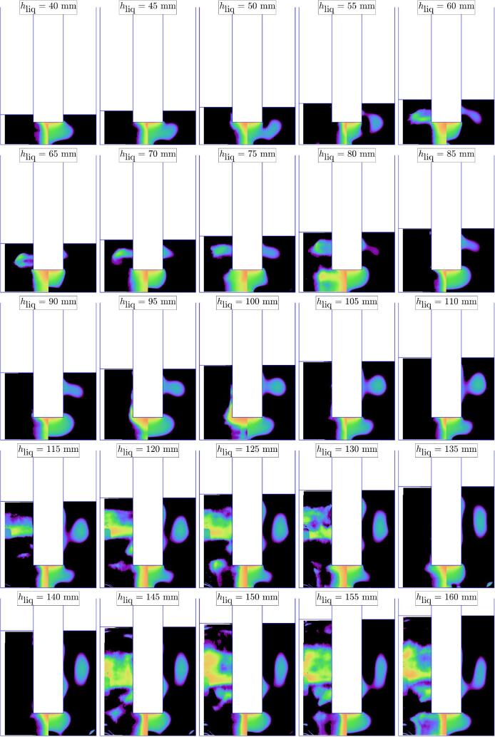
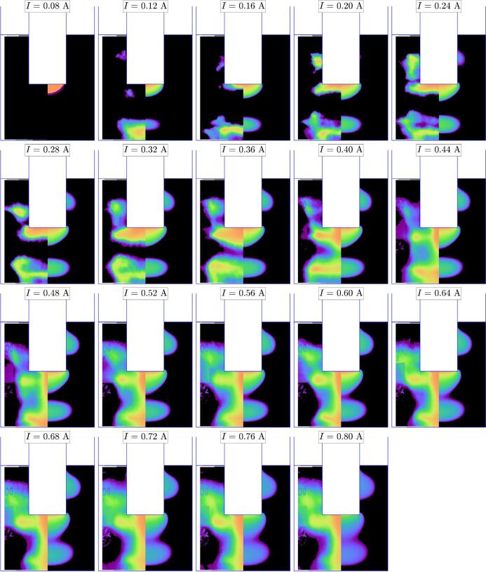
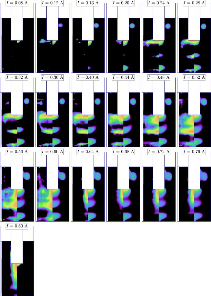
This investigation focuses on the influence of geometric factors on cavitational activity within a 20kHz sonoreactor containing water. Three vessels with different shapes were used, and the transducer immersion depth and liquid height were varied, resulting in a total of 126 experiments conducted under constant driving current. For each one, the dissipated power was quantified using calorimetry, while luminol mapping was employed to identify the shape and location of cavitation zones. The raw images of blueish light emission were transformed into false colors and corrected to compensate for refraction by the water-glass and glass-air interfaces. Additionally, all configurations were simulated using a sonoreactor model that incorporates a nonlinear propagation of acoustic waves in cavitating liquids. A systematic visual comparison between luminol maps and color-plots displaying the computed bubble collapse temperature in bubbly regions was conducted. The calorimetric power exhibited a nearly constant yield of approximately 70% across all experiments, thus validating the transducer command strategy. However, the numerical predictions consistently overestimated the electrical and calorimetric powers by a factor of roughly 2, indicating an overestimation of dissipation in the cavitating liquid model. Geometric variations revealed non-monotonic relationships between transducer immersion depth and dissipated power, emphasizing the importance of geometric effects in sonoreactor. Complex features were revealed by luminol maps, exhibiting appearance, disappearance, and merging of different luminol zones. In certain parametric regions, the luminol bright regions are reminiscent of linear eigenmodes of the water/vessel system. In the complementary parametric space, these structures either combine with, or are obliterated by typical elongated axial structures. The latter were found to coincide with an increased calorimetric power, and are conjectured to result from a strong cavitation field beneath the transducer producing acoustic streaming. Similar methods were applied to an additional set of 57 experiments conducted under constant geometry but with varying current, and suggested that the transition to elongated structures occurs above some amplitude threshold. While the model partially reproduced some experimental observations, further refinement is required to accurately account for the intricate acoustic phenomena involved.

Keywords: Acoustic cavitation; Calorimetry; Simulation; Sono-chemiluminescense; Ultrasound.

Fig. 1

Schematic of the experimental setup.

Fig. 2

Illustration of the image treatment process (applied to experiment set 2, vessel B, $h_B=190\mathrm{mm}$). (a) Original luminol figure . (b) Original luminol figure converted to false colors. The yellow lines are the deformed boundaries of the vessel and transducer, as seen by the camera, deduced from ray-tracing. (c) Image corrected against refraction. The blue lines are the real, undeformed boundaries as they would appear if there were no refraction. (d) Same as (c), symmetrized.

Fig. 3

Mechanical boundary conditions for the solid and acoustic boundary conditions for the liquid. The blue lines couple the liquid acoustics to the solid vibrations. The yellow rectangles are the piezo-electric rings.

Fig. 4

Experiments set 1: comparison between simulated and experimental electrical and calorimetric power in function of distance from transducer to bottom for the vessels A, B and C (liquid volume was 836 mL, 1818 mL, and 1767 mL for the vessels A, B and C, respectively; input current was 0.6A; and all the data points have error bars).

Fig. 5

Experiments set 1, vessel A: SCL emission (left part of images) and predicted collapse temperature field (right part of images) at different immersion depths. The input current was $I_{0,\mathrm{RMS}}=0.6\mathrm{A}$ and the liquid height computed from Eq. (1).

Fig. 6

Experiments set 1, vessel B: SCL emission (left part of images) and predicted collapse temperature field (right part of images) at different immersion depths. The input current was $I_{0,\mathrm{RMS}}=0.6\mathrm{A}$ and the liquid height computed from Eq. (1).

Fig. 7

Experiments set 1, vessel C: SCL emission (left part of images) and predicted collapse temperature field (right part of images) at different immersion depths. The input current was $I_{0,\mathrm{RMS}}=0.6\mathrm{A}$ and the liquid height computed from Eq. (1).

Fig. 8

Experiment set 2: comparison between simulated and experimental electrical and calorimetric power in function of liquid level for the vessels A, B and C (the distance between the transducer’s tip and the vessel’s bottom was 20 mm, 80 mm, and 30 mm for the vessels A, B and C, respectively; input current was 0.6A; and all the data points have error bars).

Fig. 9

Experiments set 2, vessel A: SCL emission (left part of images) and predicted collapse temperature field (right part of images) at different liquid levels. The input current was $I_{0,\mathrm{RMS}}=0.6\mathrm{A}$ and the distance between the transducer’s tip and the vessel’s bottom $h_B=20\mathrm{mm}$.

Fig. 10

Experiments set 2, vessel B: SCL emission (left part of images) and predicted collapse temperature field (right part of images) at different liquid levels. The input current was $I_{0,\mathrm{RMS}}=0.6\mathrm{A}$ and the distance between the transducer’s tip and the vessel’s bottom $h_B=80\mathrm{mm}$.

Fig. 11

Experiments set 2, vessel C: SCL emission (left part of images) and predicted collapse temperature field (right part of images) at different liquid levels. The input current was $I_{0,\mathrm{RMS}}=0.6\mathrm{A}$ and the distance between the transducer’s tip and the vessel’s bottom $h_B=30\mathrm{mm}$.

Fig. 12

Experiments set 3: comparison between simulated and experimental electrical and calorimetric power in function of input current for the vessels A, B and C (liquid volume was 836 mL, 1818 mL, and 1767 mL for the vessels A, B and C, respectively; the distance between the transducer’s tip and the vessel’s bottom was 60 mm, 110 mm, and 80 mm for the vessels A, B and C, respectively; and all the data points have error bars).

Fig. 13

Experiments set 3, vessel A: SCL emission (left part of images) and predicted collapse temperature field (right part of images) for different input currents. The distance between the transducer’s tip and the vessel’s bottom $h_B=60\mathrm{mm}$ and the liquid volume was 836ml.

Fig. 14

Experiments set 3, vessel B: SCL emission (left part of images) and predicted collapse temperature field (right part of images) for different input currents. The distance between the transducer’s tip and the vessel’s bottom $h_B=110\mathrm{mm}$ and the liquid volume was 1818ml.

Fig. 15

Experiments set 3, vessel C: SCL emission (left part of images) and predicted collapse temperature field (right part of images) for different input currents. The distance between the transducer’s tip and the vessel’s bottom $h_B=80\mathrm{mm}$ and the liquid volume was 1767ml.

Fig. A.16

Sketch of the optical system view from above. The optical axis, and all optical data are sketched in red. The camera lens is assumed equivalent to a simple thin lens with optical center $O^{\prime }$ and focal length $f=49.4\mathrm{mm}$. The vessel midplane is at distance $L=59.5\mathrm{cm}$ from sensor. A point M in the vessel mid-plane is imaged at point P on sensor, and seems to originate from point $M_{\mathrm{app}}$. The latter is located in the object plane, at distance $L_f=s_O+s_I$ from the sensor, where $s_O$ is the object distance and $s_I$ the image distance. Among all the rays travelling from M to P (pink lines), the chief ray (blue line) crosses the optical center and is undeviated.

References

1. Matouq M.A.-D., Al-Anber Z.A. Ultrason. Sonochem. 2007;14(3):393–397. - PubMed
1. Agarkoti C., Thanekar P.D., Gogate P.R. J. Environ. Manage. 2021;300 - PubMed
1. Vinatoru M. Ultrason. Sonochem. 2001;8(3):303–313. - PubMed
1. Nguele R., Okawa H. Ultrason. Sonochem. 2021;80 - PMC - PubMed
1. Chen Y., Zheng H., Truong V.N.T., Xie G., Liu Q. Ultrason. Sonochem. 2020;63 - PubMed
LinkOut - more resources