. 2023 Aug 14:12:e82850.
doi: 10.7554/eLife.82850.

Cytoarchitectonic, receptor distribution and functional connectivity analyses of the macaque frontal lobe

Affiliations

Cytoarchitectonic, receptor distribution and functional connectivity analyses of the macaque frontal lobe

Lucija Rapan et al. Elife. .

Abstract

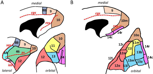
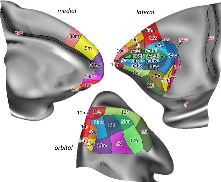
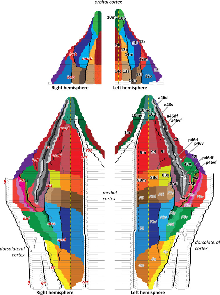
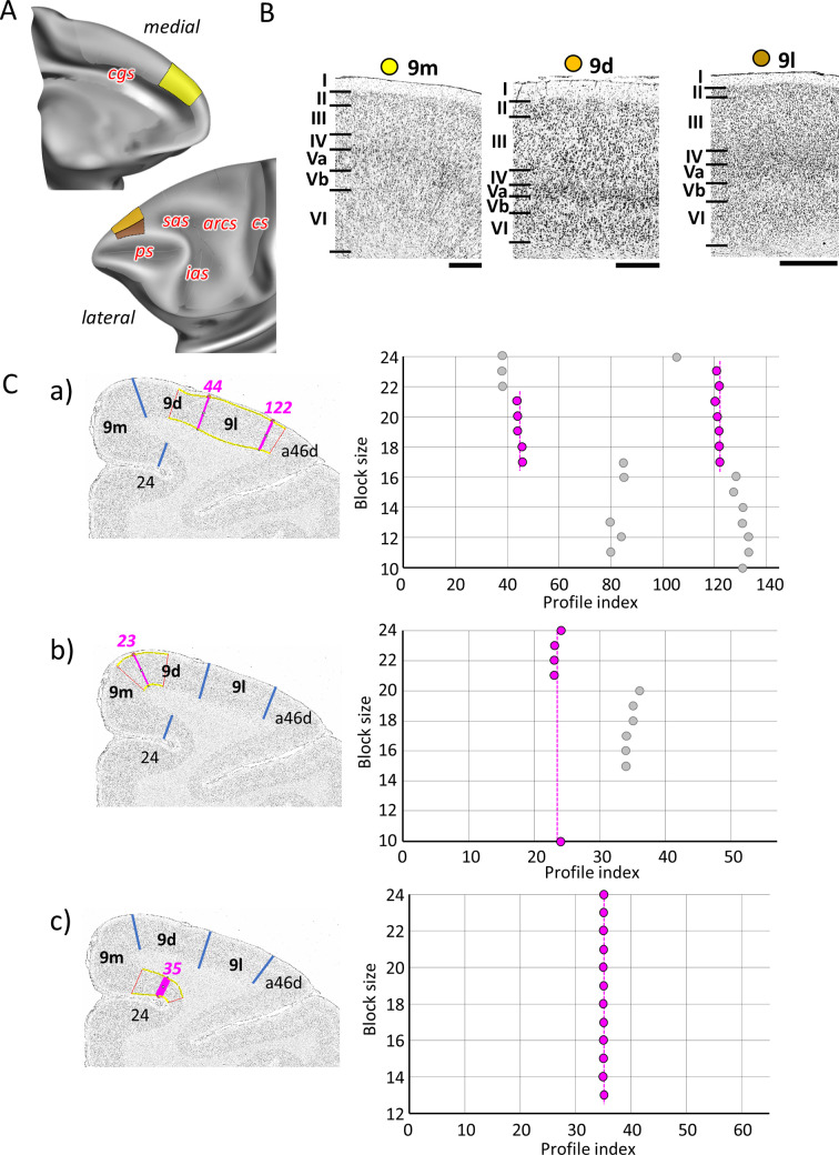
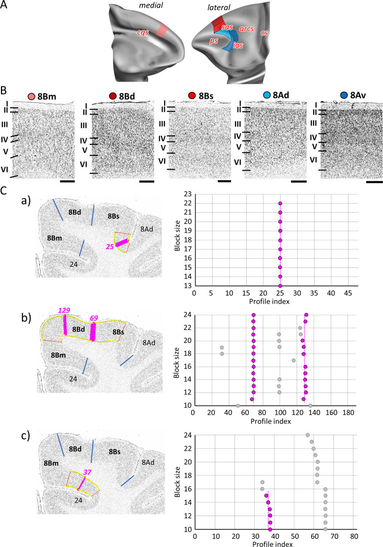
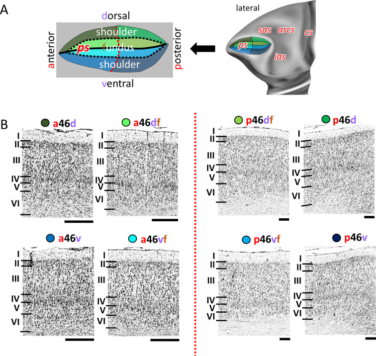
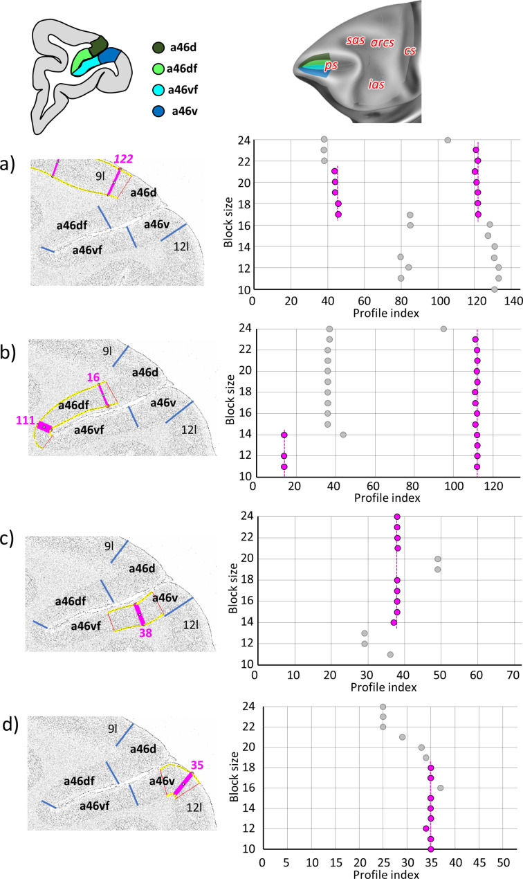
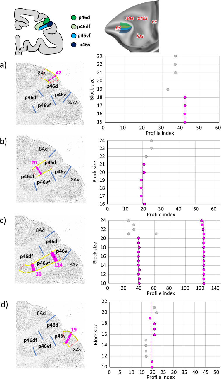
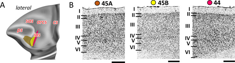
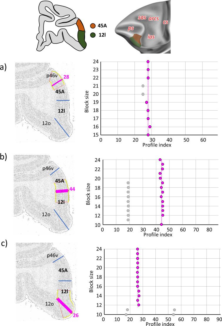
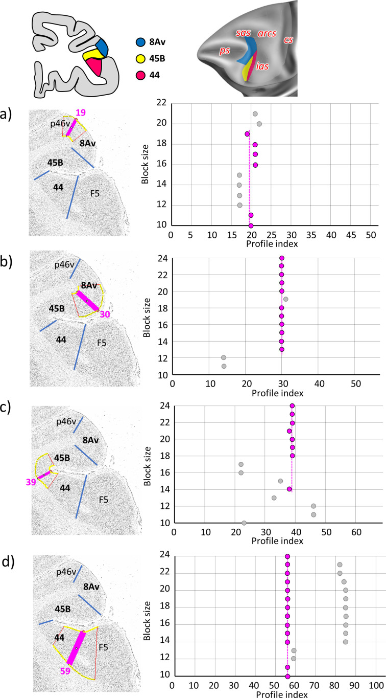
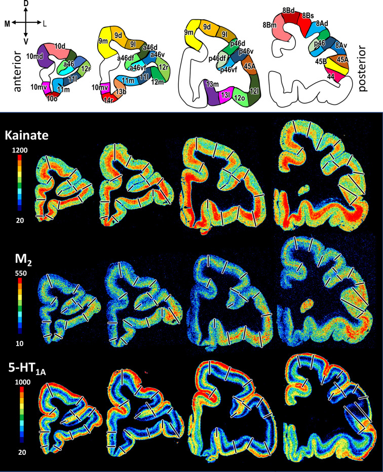
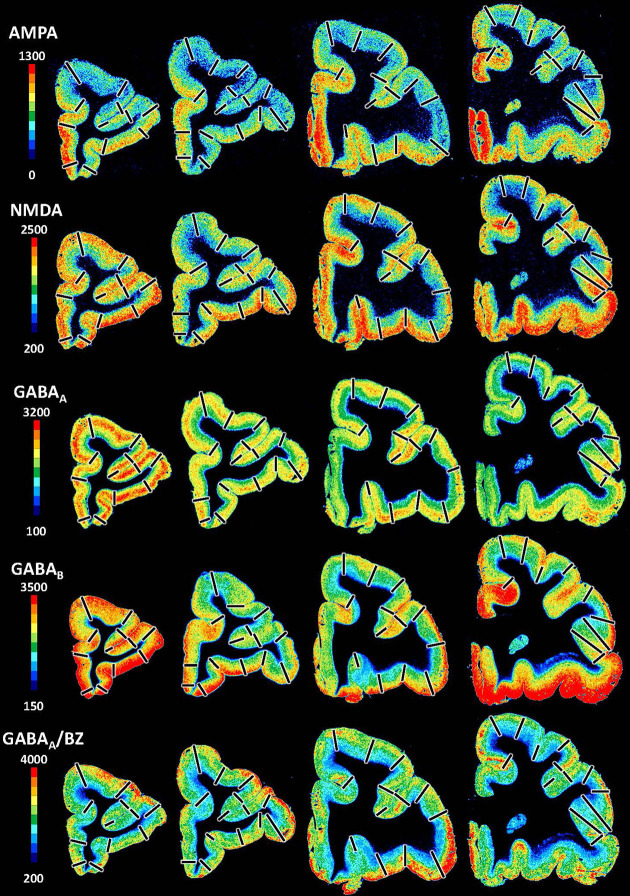
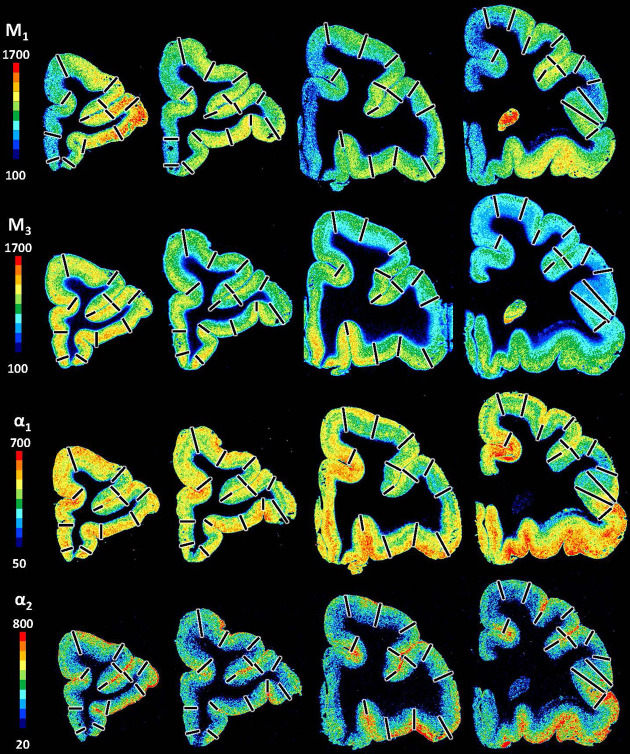
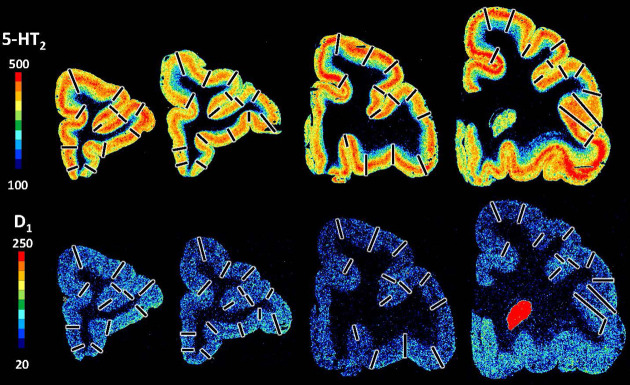
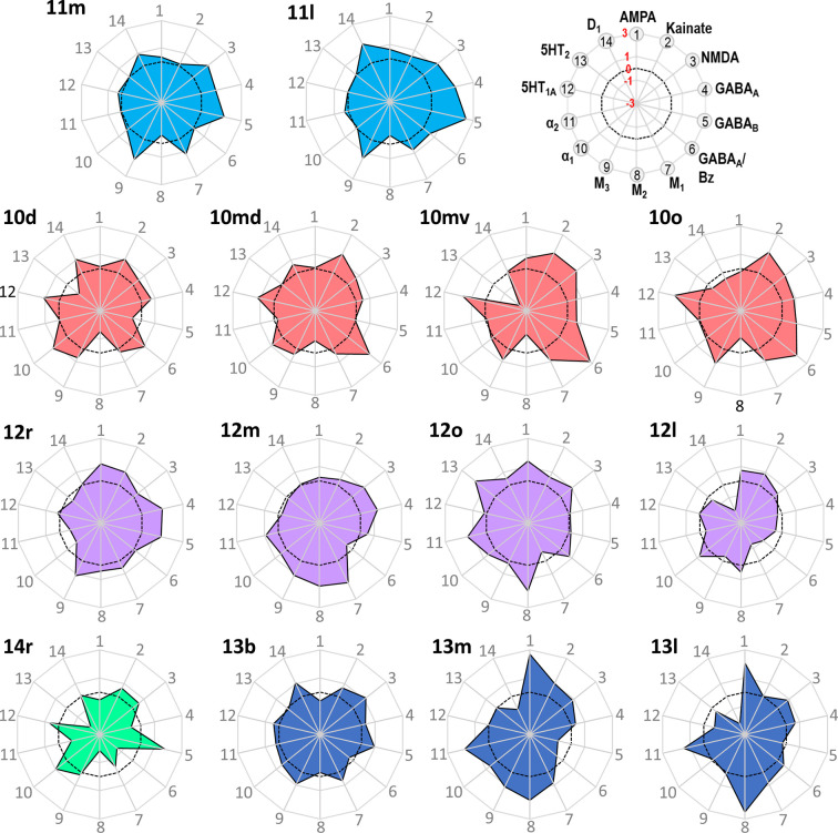
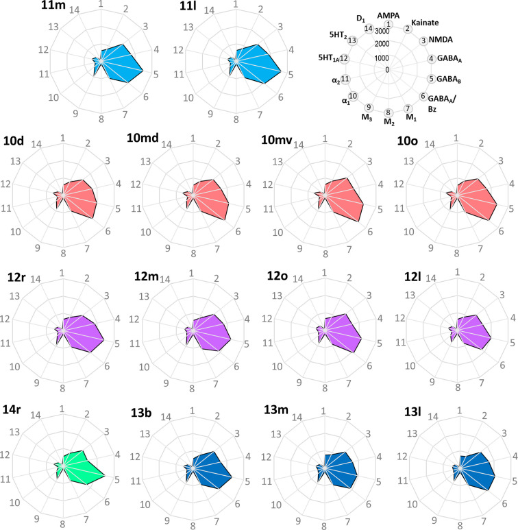
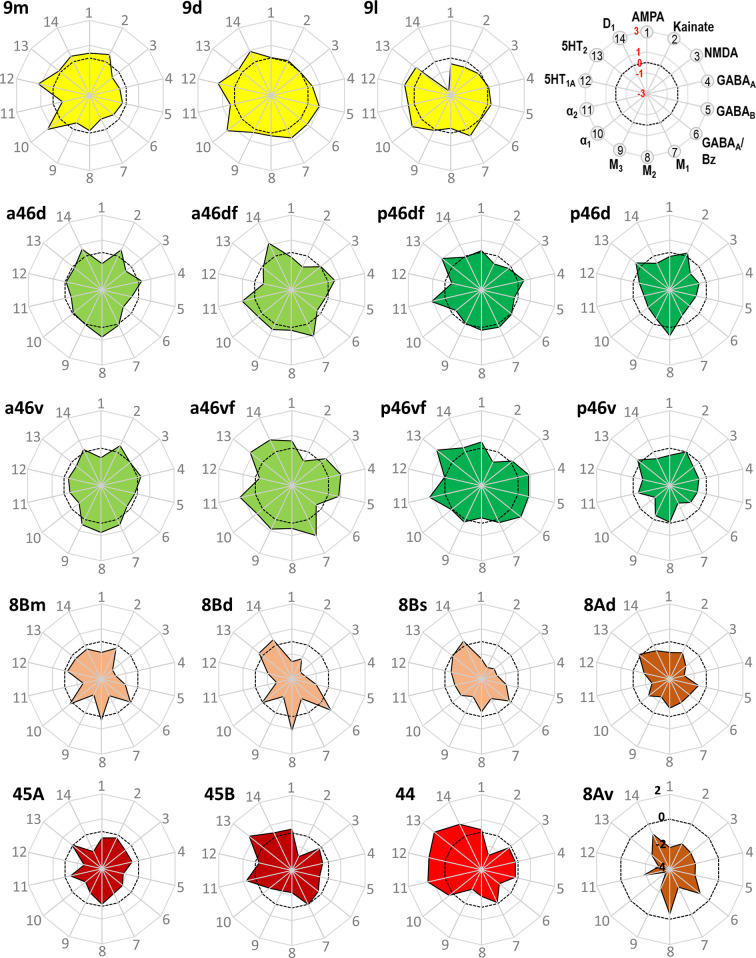
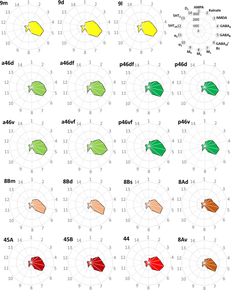
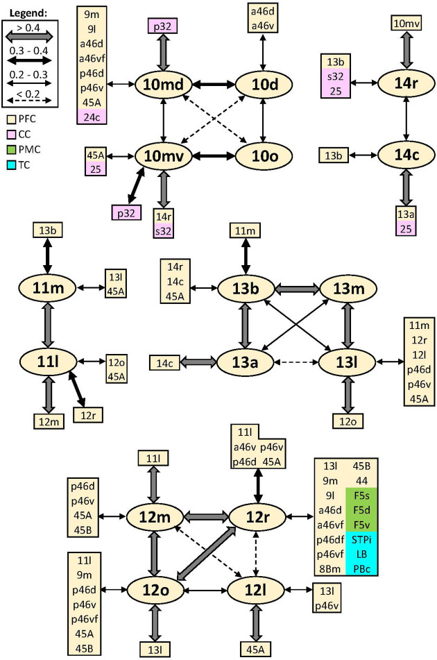
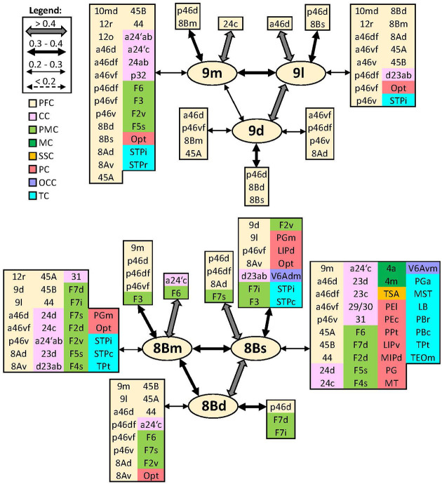
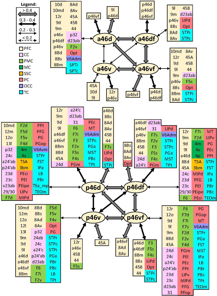
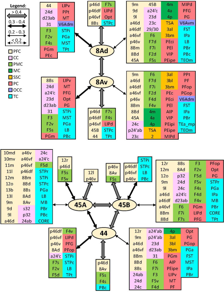
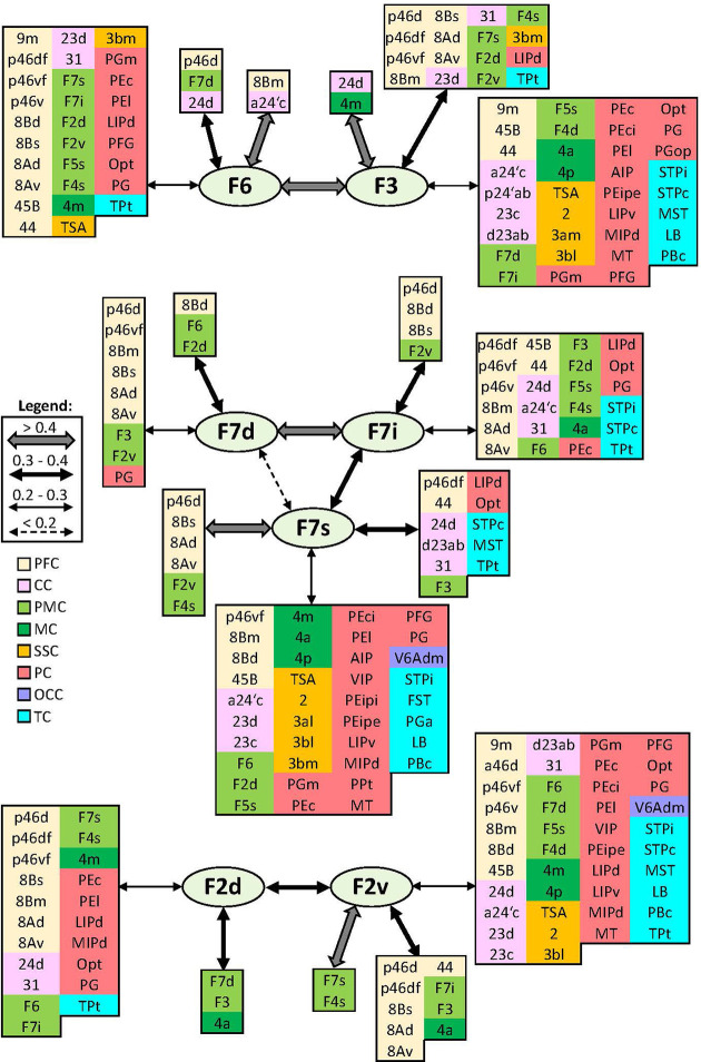
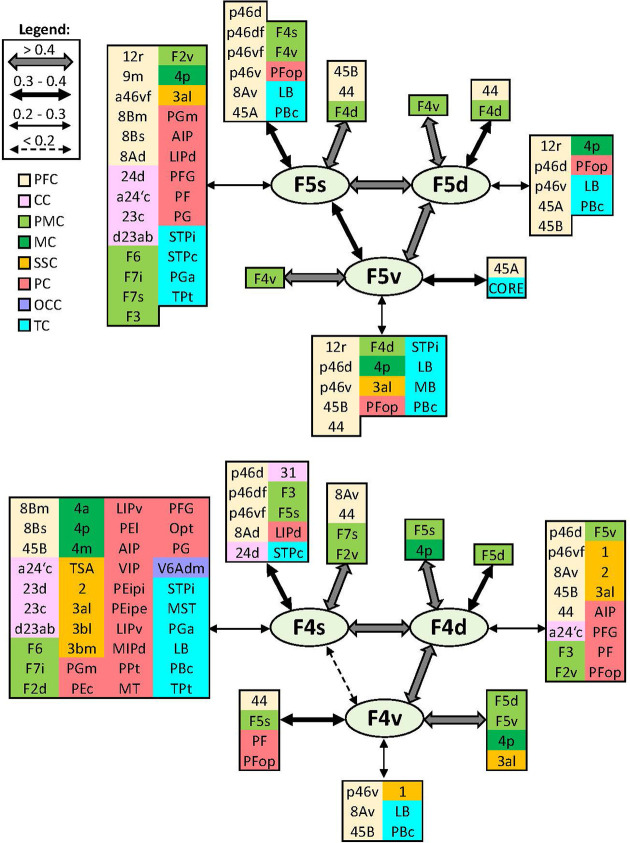
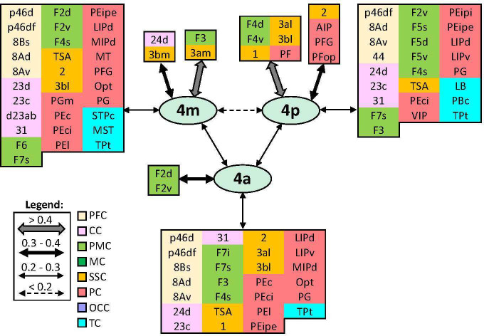
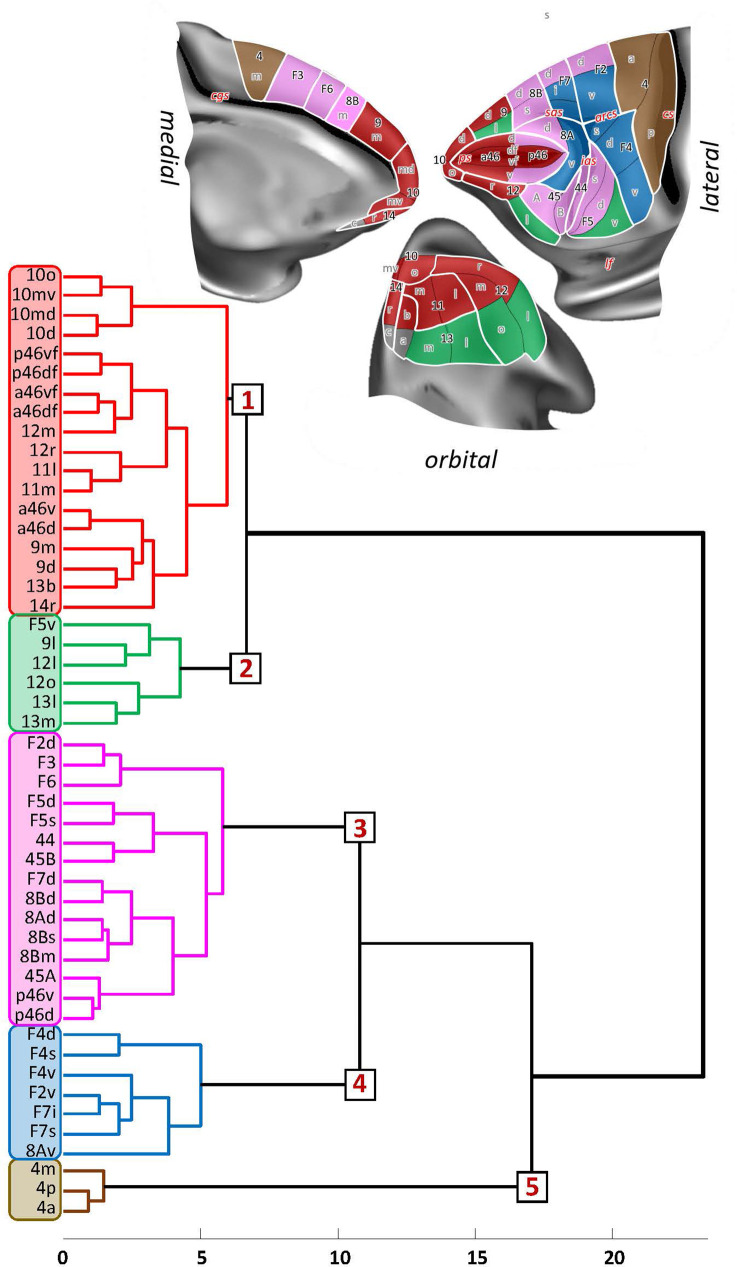
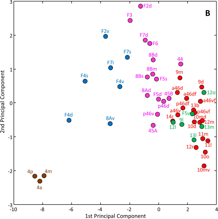
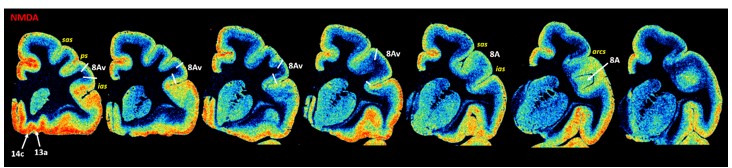
Based on quantitative cyto- and receptor architectonic analyses, we identified 35 prefrontal areas, including novel subdivisions of Walker's areas 10, 9, 8B, and 46. Statistical analysis of receptor densities revealed regional differences in lateral and ventrolateral prefrontal cortex. Indeed, structural and functional organization of subdivisions encompassing areas 46 and 12 demonstrated significant differences in the interareal levels of α2 receptors. Furthermore, multivariate analysis included receptor fingerprints of previously identified 16 motor areas in the same macaque brains and revealed 5 clusters encompassing frontal lobe areas. We used the MRI datasets from the non-human primate data sharing consortium PRIME-DE to perform functional connectivity analyses using the resulting frontal maps as seed regions. In general, rostrally located frontal areas were characterized by bigger fingerprints, that is, higher receptor densities, and stronger regional interconnections. Whereas more caudal areas had smaller fingerprints, but showed a widespread connectivity pattern with distant cortical regions. Taken together, this study provides a comprehensive insight into the molecular structure underlying the functional organization of the cortex and, thus, reconcile the discrepancies between the structural and functional hierarchical organization of the primate frontal lobe. Finally, our data are publicly available via the EBRAINS and BALSA repositories for the entire scientific community.

Keywords: cytoarchitecture; functional connectivity; macaque; motor; neuroscience; prefrontal; receptor; rhesus macaque.


Conflict of interest statement

LR, SF, MN, TX, LZ, TF, XW, KA, NP No competing interests declared

Figures

Figure 1.
Figure 1.. Schematic drawing of the medial, lateral, and orbital surfaces of the macaque prefrontal cortex depicting parcellations according to (A) Walker, 1940, and (B) Carmichael and Price, 1994.
Macroanatomical landmarks are marked with red dashed lines; cgs, cingulate sulcus; ias, inferior arcuate sulcus; ps, principal sulcus; ros, rostral orbital sulcus; sas, superior arcuate sulcus.
Figure 2.
Figure 2.. Position and extent of the prefrontal areas on the medial, lateral, and orbital views of the Yerkes19 surface.
The files with the parcellation scheme are available via EBRAINS platform of the Human Brain Project (https://search.kg.ebrains.eu/instances/Project/e39a0407-a98a-480e-9c63-4a2225ddfbe4) and the BALSA neuroimaging site (https://balsa.wustl.edu/study/7xGrm). Macroanatomical landmarks are marked in red letters, while black dashed lines mark fundus of sulci. arcs, spur of the arcuate sulcus; cgs, cingulate sulcus; cs, central sulcus; ias, inferior arcuate sulcus; lf, lateral fissure; ps, principal sulcus; sas, superior arcuate sulcus.
Figure 2—figure supplement 1.
Figure 2—figure supplement 1.. Macroanatomical landmarks (sulci labelled in red letters and dimples in green) shown on the lateral surface of the two related species of macaque monkey used in the present architectonic analyses.
Photographs of two of the postmortem brains used in this study. Brain ID DP1. (A) Macaca mulatta, and brain ID 11530 (B) Macaca fascicularis. Average surface representations of the Yerkes19. (C) Macaca mulatta template brains. arcs, spur of the arcuate sulcus; asd, anterior supracentral dimple; aspd, anterior superior principal dimple; cs, central sulcus; ias, inferior arcuate sulcus; ps, principal sulcus; pspd, posterior superior principal dimple; sas, superior arcuate sulcus; spcd, superior precentral dimple.
Figure 2—figure supplement 2.
Figure 2—figure supplement 2.. 2D flat map, based on the macroanatomical landmarks of every 40th section, displays orbital, medial, and dorsolateral hemispheric views with all defined areas within the macaque frontal lobe.
Areas are labelled on the left hemisphere, that is, prefrontal areas in black and previously mapped (pre)motor areas (Rapan et al., 2021) in grey. Due to limited space on the map, we used white arrows to mark anterior and posterior subdivisions of 46. Dashed yellow line on the hemispheres represents the midline, which separates medial and dorsolateral cortex. Black full lines mark the fundus of sulci. Macroanatomical landmarks are marked on the right hemisphere; arcs, spur of the arcuate sulcus; asd, anterior supracentral dimple; aspd, anterior superior principal dimple; cgs, cingulate sulcus; cs, central sulcus; ias, inferior arcuate sulcus; ipd, inferior principal dimple; lf, lateral fissure; lorb, lateraral orbital sulcus; morb, medial orbital sulcus; ps, principal sulcus; pspd, posterior superior principal dimple; sas, superior arcuate sulcus; spcd, superior precentral dimple.
Figure 3.
Figure 3.. Quantitative analysis of the cytoarchitecture of Walker’s area 10 (Walker, 1940).
(A) Position and extent of subdivisions of Walker’s area 10 within the hemisphere are displayed on orbital, lateral, and medial views of the Yerkes19. Macroanatomical landmarks are marked in red letters. (B) High-resolution photomicrographs show cytoarchitectonic features of areas 10d, 10md, 10mv, and 10o. Each subdivision is labelled by a coloured dot, matching the colour of the depicted area on the 3D model. (C) We confirmed cytoarchitectonic borders by a statistically testable method, where the Mahalanobis distance (MD) was used to quantify differences in the shape of profiles extracted from the region of interest. Profiles were extracted between outer and inner contour lines (yellow lines drawn between layers I/II and VI/white matter, respectively) defined on grey-level index (GLI) images of the histological sections (left column). Pink lines highlight the position of the border for which statistical significance was tested. The dot plots (right column) reveal that the location of the significant border remains constant over a large block size interval (highlighted by the red dots). (a) depicts analysis of the border between areas 10d and a46d (profile index 23); (b) depicts analysis of the border delineating dorsally located subdivisions, 10d and10md (profile index 48), as well as the medial border segregating dorsal and ventral subdivision, 10md and 10mv (profile index 127); and (c) depicts analysis of the borders between ventrally positioned subdivisions of the frontal polar region, 10mv and 10o (profile index 38) and 10o and 11m (profile index 81). Scale bar 1 mm. Roman numerals indicate cytoarchitectonic layers. arcs, spur of the arcuate sulcus; cgs, cingulate sulcus; cs, central sulcus; ias, inferior arcuate sulcus; ps, principal sulcus; sas, superior arcuate sulcus.
Figure 4.
Figure 4.. Cytoarchitecture of orbitofrontal areas.
(A) Position and extent of the orbitofrontal areas within the hemisphere are displayed on orbital, lateral, and medial views of the Yerkes19. Macroanatomical landmarks are marked in red letters. (B) High-resolution photomicrographs show cytoarchitectonic features of orbitofrontal 14r, 14c, 11m, 11l, 12r, 12m, 12l, 12o, 13b, 13a, 13m, and 13l. Each subdivision is labelled by a coloured dot, matching the colour of the depict area on the 3D model. Scale bar 1 mm. Roman numerals (and letters) indicate cytoarchitectonic layers. arcs, spur of the arcuate sulcus; cgs, cingulate sulcus; cs, central sulcus; ias, inferior arcuate sulcus; ps, principal sulcus; sas, superior arcuate sulcus.
Figure 4—figure supplement 1.
Figure 4—figure supplement 1.. Statistically testable borders (pink lines) confirmed by the quantitative analysis for the rostral orbital and ventrolateral areas 14r, 13b, 11m, 11l, 12m, and 12r.
(a) Border between 14r and 10mv (profile index 55); (b) border between 14a and 13b (profile index 28); (c) border between 13b and 11m (profile index 38); (d) borders between 11m and 11l (profile index 110) and 11l and 12m (profile index 28); (e) border between 12m and 12r (profile index 43); and (f) border between 124 and a46v (profile index 31). For details see Figure 3.
Figure 4—figure supplement 2.
Figure 4—figure supplement 2.. Statistically testable borders (pink lines) confirmed by the quantitative analysis for the caudal orbital and ventrolateral areas 14c, 13a, 13m, 13l, and 12o.
(a) Border between 25 and 14c (profile index 26); (b) border between 14c and 13a (profile index 22); (c) border between 13a and 13m (profile index 40); (d) border between 13m and 13l (profile index 59); (e) border between 13l and 12o (profile index 56); and (f) border between 12o and 12l (profile index 76). For details see Figure 3.
Figure 5.
Figure 5.. Quantitative analysis of the cytoarchitecture of Walker’s area 9 (Walker, 1940).
(A) Position and extent of the rostral medial and dorsolateral prefrontal areas within the hemisphere are displayed on lateral and medial views of the Yerkes19. Macroanatomical landmarks are marked in red letters. (B) High-resolution photomicrographs show cytoarchitectonic features of areas 9m, 9d, and 9l. Each subdivision is labelled by a coloured dot, matching the colour of the depict area on the 3D model. (C) We confirmed cytoarchitectonic borders by statistically testable method (for details see Figure 3). (a) depicts analysis of the borders between area a46d and 9l (profile index 122), as well as 9l and 9d (profile index 44); (b) depicts analysis of the border between dorsal and medial subdivision, 9d and 9m (profile index 44); and (c) depicts analysis of the border distinguishing medial subdivision 9m from cingulate cortex, area 24 (profile index 35). Scale bar 1 mm. Roman numerals (and letters) indicate cytoarchitectonic layers. arcs, spur of the arcuate sulcus; cgs, cingulate sulcus; cs, central sulcus; ias, inferior arcuate sulcus; ps, principal sulcus; sas, superior arcuate sulcus.
Figure 6.
Figure 6.. Quantitative analysis of the cytoarchitecture of Walker’s area 8B (Walker, 1940).
(A) Position and the extent of the caudal medial and dorsolateral prefrontal areas within the hemisphere are displayed on lateral and medial views of the Yerkes19. Macroanatomical landmarks are marked in red. (B) High-resolution photomicrographs show cytoarchitectonic features of areas 8B (8Bm, 8Bd, 8Bs) and 8A (8Ad, 8Av). Each subdivision is labelled by a coloured dot, matching the colour of the depict area on the 3D model. (C) We confirmed cytoarchitectonic borders of new 8B subdivisions by statistically testable method (for details see Figure 3). (a) depicts analysis of the border that separates new subdivisions 8Bs from neighbouring area 8Ad (profile index 25); (b) depicts analysis of the borders which delineate area 8Bd from surrounding areas 8Bs and 8Bm (profile index 69), as well as 8Bd and 8Bm (profile index 129); and (c) depicts analysis of the border distinguishing medial subdivision 8Bm from cingulate cortex, area 24 (profile index 37). Statistically testable borders for area 8Ad (adjacent to p46d) shown in Figure 7—figure supplement 2 and for area 8Av borders can be seen in the Figure 8—figure supplement 2. Scale bar 1 mm. Roman numerals (and letters) indicate cytoarchitectonic layers. arcs, spur of the arcuate sulcus; cgs, cingulate sulcus; cs, central sulcus; ias, inferior arcuate sulcus; ps, principal sulcus; sas, superior arcuate sulcus.
Figure 7.
Figure 7.. Cytoarchitecture of Walker’s area 46 (Walker, 1940).
(A) Position and the extent of areas located within and around the ps, are displayed on lateral view of the Yerkes19. Additionally, schematic drowning demonstrates how identified subdivisions are labelled with letters highlighted in red. Macroanatomical landmarks are marked in red letters. Black line indicates fundus, black dotted line marks border between shoulder and fundus region, and red dotted line separates anterior and posterior portion of sulcus. (B) High-resolution photomicrographs show cytoarchitectonic features of anterior areas of 46 (a46d, a46df, a46vf, a46v) and posterior ones (p46d, p46df, p46vf, p46v), separated by red dashed line. Each subdivision is labelled by a coloured dot, matching the colour of the depict area on the 3D model. Scale bar 1 mm. Roman numerals indicate cytoarchitectonic layers. arcs, spur of the arcuate sulcus; cs, central sulcus; ias, inferior arcuate sulcus; ps, principal sulcus; sas, superior arcuate sulcus.
Figure 7—figure supplement 1.
Figure 7—figure supplement 1.. Statistically testable borders (pink lines) confirmed by the quantitative analysis for the rostral region of the ps, occupied by the anterior subdivisions of area 46; a46d, a46df, a46vf, and a46v.
(a) Border between 9l and a46d (profile index 122); (b) borders between a46d and a46df (profile index 16) and a46df and a46vf (profile index 111); (c) border between ap46vf and a46v (profile index 38); and (d) border between a46v and 12l (profile index 35). For details see Figure 3.
Figure 7—figure supplement 2.
Figure 7—figure supplement 2.. Statistically testable borders (pink lines) confirmed by the quantitative analysis for the caudal region of the ps, occupied by the posterior subdivisions of area 46; p46d, p46df, p46vf, and p46v.
(a) Border between 8Ad and p46d (profile index 42); (b) border between p46d and p46df (profile index 20); (c) borders between p46df and p46vf (profile index 39) and p46vf and p46v (profile index 124); and (d) border between p46v and 8Av (profile index 19). For details see Figure 3.
Figure 8.
Figure 8.. Cytoarchitecture of areas 44 and 45.
(A) Position and the extent of the posterior ventrolateral areas within the hemisphere are displayed on lateral view of the Yerkes19. Macroanatomical landmarks are marked in red letters. (B) High-resolution photomicrographs show cytoarchitectonic features of areas 44 and 45 (45A, 45B). Each subdivision is labelled by a coloured dot, matching the colour of the depict area on the 3D model. Scale bar 1 mm. Roman numerals indicate cytoarchitectonic layers. arcs, spur of the arcuate sulcus; cs, central sulcus; ias, inferior arcuate sulcus; ps, principal sulcus; sas, superior arcuate sulcus.
Figure 8—figure supplement 1.
Figure 8—figure supplement 1.. Statistically testable borders (pink lines) confirmed by the quantitative analysis for the caudal ventrolateral area 12l and dorsally adjacent area 45A.
(a) Border between p46v and 45A (profile index 28); (b) border between 45A and 12l (profile index 44); and (c) border between 12l and 12o (profile index 26). For details see Figure 3.
Figure 8—figure supplement 2.
Figure 8—figure supplement 2.. Statistically testable borders (pink lines) confirmed by the quantitative analysis for the caudal ventrolateral cortex; areas 8Av, 45B, and 44.
(a) Border between p46v and 8Av (profile index 19); (b) border between 8Av and 45B (profile index 30); (c) border between 45B and 44 (profile index 39); and (d) border between 44 and F5 (prolfile index 59). For details see Figure 3.
Figure 9.
Figure 9.. Exemplary sections depicting the distribution of kainate, M2 and 5-HT1A receptors in coronal sections through a macaque hemisphere.
The colour bar, positioned left to the autoradiographs, codes receptor densities in fmol/mg protein, and borders are indicated by black lines. The four schematic drawings at the top represent the distinct rostro-caudal levels and show the position of all prefrontal areas defined. C, caudal; D, dorsal; R, rostral; V, ventral.
Figure 9—figure supplement 1.
Figure 9—figure supplement 1.. Exemplary sections depicting the distribution of the remaining receptor types, that is, of glutamate (AMPA, kainate, NMDA) and gamma-aminobutyric acid (GABA) (GABAA, GABAB, GABAA-associated benzodiazepine binding sites – BZ) receptors, in coronal sections through a macaque hemisphere.
The colour bar positioned left to the autoradiographs codes values of receptor densities in fmol/mg protein, and borders are indicated by the black lines.
Figure 9—figure supplement 2.
Figure 9—figure supplement 2.. Exemplary sections depicting the distribution of the remaining receptor types, that is, acetylcholine (M1, M2, M3) and noradrenalin (α1, α2) receptors in coronal sections through a macaque hemisphere.
The colour bar positioned left to the autoradiographs codes values of receptor densities in fmol/mg protein, and borders are indicated by the black lines.
Figure 9—figure supplement 3.
Figure 9—figure supplement 3.. Exemplary sections depicting the distribution of the remaining receptor types, that is, serotonin (5HT2) and dopamine (D1) receptors in coronal sections through a macaque hemisphere.
The colour bar positioned left to the autoradiographs codes values of receptor densities in fmol/mg protein, and borders are indicated by the black lines.
Figure 10.
Figure 10.. Normalized receptor fingerprints of the frontopolar and orbital areas.
Black dotted line on the plot represents the mean value over all areas for each receptor. Receptors displaying a negative z-score are indicative of absolute receptor densities which are lower than the average of that specific receptor over all examined areas. The opposite is true for positive z-scores. Labelling of different receptor types, as well as the axis scaling, is identical for each area plot, which is specified in the polar plot on the top of the figure.
Figure 10—figure supplement 1.
Figure 10—figure supplement 1.. Receptor fingerprints of the frontopolar and orbital areas.
Absolute receptor densities are given in fmol/mg protein. The positions of the different receptor types and the axis scaling are identical in all areas, and specified in the polar plot on the top of the figure.
Figure 11.
Figure 11.. Normalized receptor fingerprints of the medial, dorsolateral, lateral, and ventrolateral areas.
Black dotted line on the plot represents the mean value over all areas for each receptor. Receptors displaying a negative z-score are indicative of absolute receptor densities which are lower than the average of that specific receptor over all examined areas. The opposite is true for positive z-scores. Labelling of different receptor types, as well as the axis scaling, is identical for each area plot, which is specified in the polar plot on the top of the figure. Due to the low receptor densities measured in area 8Av, scaling for its fingerprint is adjusted and shown directly on the corresponding polar plot.
Figure 11—figure supplement 1.
Figure 11—figure supplement 1.. Receptor fingerprints of the medial, dorsolateral, lateral, and ventrolateral areas.
Absolute receptor densities are given in fmol/mg protein. The positions of the different receptor types and the axis scaling are identical in all areas, and specified in the polar plot on the top of the figure.
Figure 12.
Figure 12.. Schematic summary of the functional connectivity analysis between subdivisions of areas 10, 14, 11, 13, and 12.
Legend shows the strength of the functional connectivity coefficient (z) is coded by the appearance (wider-thinner-doted) of the connecting arrows. Areas related to different brain regions are marked on the scheme with distinct colours; prefrontal cortex (PFC) in light yellow, cingulate cortex (CC) in pink, premotor cortex (PMC) in light green, and temporal cortex (TC) in light blue.
Figure 13.
Figure 13.. Schematic summary of the functional connectivity analysis between subdivisions of areas 9 and 8B.
Legend shows the strength of the functional connectivity coefficient (z) is coded by the appearance (wider-thinner-doted) of the connecting arrows. Areas related to different brain region are marked on the scheme with distinct colours; prefrontal cortex (PFC) in light yellow, cingulate cortex (CC) in pink, premotor cortex (PMC) in light green, motor cortex (MC) in dark green, somatosensory cortex (SSC) in orange, parietal cortex (PC) in red, occipital cortex (OCC) in purple, and temporal cortex (TC) in light blue.
Figure 14.
Figure 14.. Schematic summary of the functional connectivity analysis between subdivisions of areas 46, rostral areas ‘a46,’ and caudal ones ‘p46’.
Legend shows the strength of the functional connectivity coefficient (z) is coded by the appearance (wider-thinner-doted) of the connecting arrows. Areas related to different brain region are marked on the scheme with distinct colours; prefrontal cortex (PFC) in light yellow, cingulate cortex (CC) in pink, premotor cortex (PMC) in light green, motor cortex (MC) in dark green, somatosensory cortex (SSC) in orange, parietal cortex (PC) in red, occipital cortex (OCC) in purple, and temporal cortex (TC) in light blue.
Figure 15.
Figure 15.. Schematic summary of the functional connectivity analysis between subdivisions of areas 8A and 45, and area 44.
Legend shows the strength of the functional connectivity coefficient (z) is coded by the appearance (wider-thinner-doted) of the connecting arrows. Areas related to different brain region are marked on the scheme with distinct colours; prefrontal cortex (PFC) in light yellow, cingulate cortex (CC) in pink, premotor cortex (PMC) in light green, motor cortex (MC) in dark green, somatosensory cortex (SSC) in orange, parietal cortex (PC) in red, occipital cortex (OCC) in purple, and temporal cortex (TC) in light blue.
Figure 16.
Figure 16.. Schematic summary of the functional connectivity analysis between subdivisions of premotor areas F7 and F2, and areas F3 and F6.
Legend shows the strength of the functional connectivity coefficient (z) is coded by the appearance (wider-thinner-doted) of the connecting arrows. Areas related to different brain region are marked on the scheme with distinct colours; prefrontal cortex (PFC) in light yellow, cingulate cortex (CC) in pink, premotor cortex (PMC) in light green, motor cortex (MC) in dark green, somatosensory cortex (SSC) in orange, parietal cortex (PC) in red, occipital cortex (OCC) in purple, and temporal cortex (TC) in light blue.
Figure 17.
Figure 17.. Schematic summary of the functional connectivity analysis between subdivisions of premotor areas F5 and F4.
Legend shows the strength of the functional connectivity coefficient (z) is coded by the appearance (wider-thinner-doted) of the connecting arrows. Areas related to different brain region are marked on the scheme with distinct colours; prefrontal cortex (PFC) in light yellow, cingulate cortex (CC) in pink, premotor cortex (PMC) in light green, motor cortex (MC) in dark green, somatosensory cortex (SSC) in orange, parietal cortex (PC) in red, occipital cortex (OCC) in purple, and temporal cortex (TC) in light blue.
Figure 18.
Figure 18.. Schematic summary of the functional connectivity analysis between subdivisions of primary motor areas 4.
Legend shows the strength of the functional connectivity coefficient (z) is coded by the appearance (wider-thinner-doted) of the connecting arrows. Areas related to different brain region are marked on the scheme with distinct colours; prefrontal cortex (PFC) in light yellow, cingulate cortex (CC) in pink, premotor cortex (PMC) in light green, motor cortex (MC) in dark green, somatosensory cortex (SSC) in orange, parietal cortex (PC) in red, occipital cortex (OCC) in purple, and temporal cortex (TC) in light blue.
Figure 19.
Figure 19.. Receptor-driven hierarchical clustering of the receptor fingerprints in the macaque frontal lobe.
The analyses include 33 of the 35 areas identified in this study (for areas 14c and 13a was not possible to extract receptor densities due to technical limitations), as well as 16 areas of the primary motor and premotor cortex identified in a previous study (Rapan et al., 2021) carried out on the same monkey brains. Above the hierarchical dendrogram, the extent and location of the five clusters are depicted on the medial, lateral, and orbital surface of the Yerkes19 atlas. Clusters are colour coded based on the corresponding colour on the dendrogram.
Figure 20.
Figure 20.. Principal component analysis (variance 79.8%) of the receptor fingerprints, where the k-means analysis showed five as the optimal number of clusters.
Author response image 1.

Update of

  • doi: 10.1101/2022.06.27.497757

Similar articles

Cited by

References

    1. Adachi Y, Osada T, Sporns O, Watanabe T, Matsui T, Miyamoto K, Miyashita Y. Functional connectivity between anatomically unconnected areas is shaped by collective network-level effects in the macaque cortex. Cerebral Cortex. 2012;22:1586–1592. doi: 10.1093/cercor/bhr234. - DOI - PubMed
    1. Amiez C, Petrides M. Anatomical organization of the eye fields in the human and non-human primate frontal cortex. Progress in Neurobiology. 2009;89:220–230. doi: 10.1016/j.pneurobio.2009.07.010. - DOI - PubMed
    1. Andersen RA, Asanuma C, Essick G, Siegel RM. Corticocortical connections of anatomically and physiologically defined subdivisions within the inferior parietal lobule. The Journal of Comparative Neurology. 1990a;296:65–113. doi: 10.1002/cne.902960106. - DOI - PubMed
    1. Andersen RA, Bracewell RM, Barash S, Gnadt JW, Fogassi L. Eye position effects on visual, memory, and saccade-related activity in areas LIP and 7A of macaque. The Journal of Neuroscience. 1990b;10:1176–1196. doi: 10.1523/JNEUROSCI.10-04-01176.1990. - DOI - PMC - PubMed
    1. Arnsten AF, Goldman-Rakic PS. Alpha 2-adrenergic mechanisms in prefrontal cortex associated with cognitive decline in aged nonhuman primates. Science. 1985;230:1273–1276. doi: 10.1126/science.2999977. - DOI - PubMed

Publication types