Global methane emissions from rivers and streams

Abstract

Methane (CH₄) is a potent greenhouse gas and its concentrations have tripled in the atmosphere since the industrial revolution. There is evidence that global warming has increased CH₄ emissions from freshwater ecosystems^1,2, providing positive feedback to the global climate. Yet for rivers and streams, the controls and the magnitude of CH₄ emissions remain highly uncertain^3,4. Here we report a spatially explicit global estimate of CH₄ emissions from running waters, accounting for 27.9 (16.7-39.7) Tg CH₄ per year and roughly equal in magnitude to those of other freshwater systems^5,6. Riverine CH₄ emissions are not strongly temperature dependent, with low average activation energy (E_M = 0.14 eV) compared with that of lakes and wetlands (E_M = 0.96 eV)¹. By contrast, global patterns of emissions are characterized by large fluxes in high- and low-latitude settings as well as in human-dominated environments. These patterns are explained by edaphic and climate features that are linked to anoxia in and near fluvial habitats, including a high supply of organic matter and water saturation in hydrologically connected soils. Our results highlight the importance of land-water connections in regulating CH₄ supply to running waters, which is vulnerable not only to direct human modifications but also to several climate change responses on land.

Fig. 1. Global patterns of CH₄ in rivers and streams.

a,b, Modelled yearly average CH₄ concentrations (a) and emissions (b) in rivers and streams. Data have been aggregated in hexagonal bins, and the size of each hexagon is rescaled with runoff, to better visualize patterns in areas with high coverage of running waters. Areas with runoff greater than 1,500 mm per year have full-sized hexagons; hexagons in areas with runoff of 500 mm per year have been reduced by 10%; and hexagons with a runoff less than 50 mm per year have been reduced by 50%. The model could not be applied in Greenland and Antarctica, which are shown in dark grey.

Fig. 2. Main drivers of CH₄ concentrations in streams.

a, The 20 most important variables in the random forest model. The x axis shows the median importance across all monthly models (n = 12), with error lines representing standard deviation (s.d.); note the square-root transformation of the x axis. The line inside each bar is the partial dependence, which represents the marginal effect of a given feature (x axis) on predicted CH₄ concentrations (y axis). These lines are a simplification of a more detailed version (Supplementary Information). b, CH₄ concentrations of some site categories from GRiMeDB were excluded from the model as they were not captured in the hydrological model or were targeted observations not representative of catchment properties (Methods). The underlying jittered points represent all other observations in GRiMeDB, with the dashed line representing the average. Each category is colour-coded, with the black dot and a line representing the mean ± s.d.

Fig. 3. Seasonal patterns of CH₄ emissions.

Left: total monthly CH₄ emissions for each latitudinal band (10° bins), with the colour representing total river area. Right: total yearly emissions for each latitudinal band. In the left panel, the y axis is square-root transformed, and the colour scale is log transformed.

Fig. 4. Temperature dependence of diffusive CH₄ emissions.

a, The relationship of water temperature with measured diffusive CH₄ emissions in GRiMeDB coloured by latitude. The solid coloured lines are linear fits for sites that have more than 20 observations and the black solid line is the linear model for all data. The dashed black line represents the slope from the average activation energy of other aquatic systems from ref. . The x axis shows the standardized temperature following ref. , where k is the Boltzmann constant, T is the water temperature in kelvin and T_c is 15 °C. The colour scale shows the absolute values of latitudinal decimal degrees. b, A kernel density plot (y axis represents the relative number of observations) of the apparent activation energy—that is, the slope of the lines in a—for rivers (this study) and other freshwater systems compiled in ref. . The vertical dashed line shows the zero x intercept.

Extended Data Fig. 1. Observations in GRiMeDB and their spatial representativeness.

Map of the globle showing the location of methane concentration observations in the database for each month (black points). The number in each panel denotates the total number of observations available each month, after aggregating temporal data for each subcatchment in GRADES. Light blue shows the snow or ice cover, and red polygons represent areas where the monthly model is extrapolating predictions (See section “Random forest modelling” in the main text for further explanation).

Extended Data Fig. 2. Performance of the random forest model.

(a) Predicted versus observed methane (CH₄) concentrations of the test dataset for each month, with the black solid line showing the 1:1 line. Inside the plot is shown the R² of the linear regression and the root mean square error (RMSE). (b) Residuals of the random forest model for predicted methane (CH₄) concentrations of the test dataset for each month. The black solid line is the x axis for y = 0.

Extended Data Fig. 3. Monthly global patterns of methane (CH₄) concentrations.

Predicted CH₄ concentrations for the globe, using a random forest model for each month. Light blue areas indicate snow or ice cover. The model was not applied in Greenland (in dark grey) and Antarctica (not shown) due to lack of data coverage for many predictors.

Extended Data Fig. 4. Uncertainty in river methane (CH₄) prediction.

Map of the standard deviation (SD) of the modelled CH₄ concentrations. The SD was obtained for each month and presented as a yearly average for this map. The model was not applied in Greenland (shown in dark grey) and Antarctica (not shown).

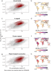
Extended Data Fig. 5. The effect of different correction methods for modeling methane (CH₄) concentration ~ flux relationships.

Uncorrected model estimates result in a large number of flux observations which are larger than observations reported in the empirical dataset. Plots in the left column provide a comparison between modelled and actual (observed) flux-concentration relationships. Red contours represent the density of modelled fluxes and concentrations, while grey contours represent the density of empirical observations available in GRiMeDB (n = 4,052), with the lowest contours containing 95% of values. The maps in the right column illustrate modelled fluxes, with mountain areas highlighted as light grey, hollow polygons (from ref. ); note the different scales for each row. Ideally, the modelled and empirical obervations of the concentration ~ flux relationship should overlap, but do not, as seen in (a), leading us to explore multiple corrections. Capping gas transfer velocity (k) (c, d) at 35 m per day does little to correct this artefact, nor does capping flux estimates above 2 standard deviations of the global population (e,f). In contrast, the river reach footprint correction avoids particularly the high fluxes at low concentrations and better represents the distribution of empirical observations (g, h). See methods section “Uncertainty and refinement of the estimate” for a detailed discussion of this issue and the approach selected.

Extended Data Fig. 6. Temperature relationship of ebullitive methane (CH₄) fluxes.

Relationship between ebullitive CH₄ fluxes and temperature in GRiMeDB. Here k is the Boltzmann constant, T is water temperature in Kelvin, and T_c is 15 °C (average water temperature in GRiMeDB). The total number of observations and model fit are shown in the figure, although the model is non-significant.

Extended Data Fig. 7. Assessment of ebullitive methane (CH₄) emissions.

Simultaneous observations of diffusive and ebullitive emissions from GRiMeDB were measured simultaneously. (a) illustrates the overall magnitude of the emissions, with the density plots (dark and light blue) showing the distribution and dot plots showing each observation. The large black dot represents the median value (n = 296). (b) shows the relationship between diffusive and ebullitive emissions, where each site with more than one measurement has a unique categorical color (number of sites = 93). The solid line is a linear model fit (model fit and statistics reported in the upper left corner of the plot) with the shaded polygon representing the 95% prediction interval, and the dashed line represents the 1:1 ratio.

Extended Data Fig. 8. Sensitivity analysis of the global methane (CH₄) diffusive estimate.

The dark grey vertical line illustrates the mean estimate of global emissions, with lighter shades representing the 50, 75 and 95 % quantiles of the Monte Carlo simulation. The sensitivity analysis was performed for each flux parameter (gas transfer velocity, CH₄ concentration, river area) by increasing (blue) or decreasing (red) a parameter by 1 SD, then re-running the Monte Carlo simulation. Vertical coloured central lines show the mean values, with the rectangles decreasing in size showing the 50, 75 and 95 % percentiles. Thin vertical lines show the individual replicates of the Monte Carlo simulation for each experiment as well as for the main estimate (grey, bottom). Note that the uncertainty of the Monte Carlo simulation is highly sensitive to the uncertainty considered for each parameter, and thus it may change if other models are used.

Extended Data Fig. 9. Comparison of modelled versus directly measured diffusive methane (CH₄) emissions.

(a) Modelled diffusive CH₄ fluxes in GRADES reaches where an empirical measurement is available in GRiMeDB. Measured fluxes span seven orders of magnitude while modelled fluxes are more constrained (2 orders of magnitude). One potential source of the discrepancy is the difference in gas transfer velocities (k) between the measured and predicted values, given that the vast majority of flux observations in GRiMeDB are measurements from a single day in a relatively short reach, while the modelled fluxes use monthly modelled discharge averages along a long river reach (4–6 km). When selecting pairs of observations with comparable k values, indicating that the hydrological conditions between the modelled and observed value are similar (predicted k is between 0.5 and 1.5 times the measured k; black points in (b)), the relationship between modelled and measured fluxes is evident. Dashed line in both panels is the 1:1 line, and note the change in the axis in panel (b).

References

1. Yvon-Durocher, G. et al. Methane fluxes show consistent temperature dependence across microbial to ecosystem scales. Nature507, 488–491 (2014). - PubMed
1. Zhu, Y. et al. Disproportionate increase in freshwater methane emissions induced by experimental warming. Nat. Clim. Change10, 685–690 (2020).
1. Stanley, E. H. et al. The ecology of methane in streams and rivers: patterns, controls, and global significance. Ecol. Monogr.86, 146–171 (2016).
1. Rosentreter, J. A. et al. Half of global methane emissions come from highly variable aquatic ecosystem sources. Nat. Geosci.14, 225–230 (2021).
1. Johnson, M. S. et al. Spatiotemporal methane emission from global reservoirs. J. Geophys. Res. Biogeosci.126, e2021JG006305 (2021).
Publication types