Genetic insights into human cortical organization and development through genome-wide analyses of 2,347 neuroimaging phenotypes

Abstract

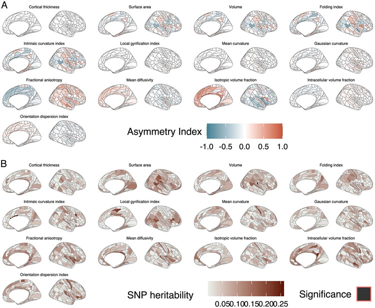
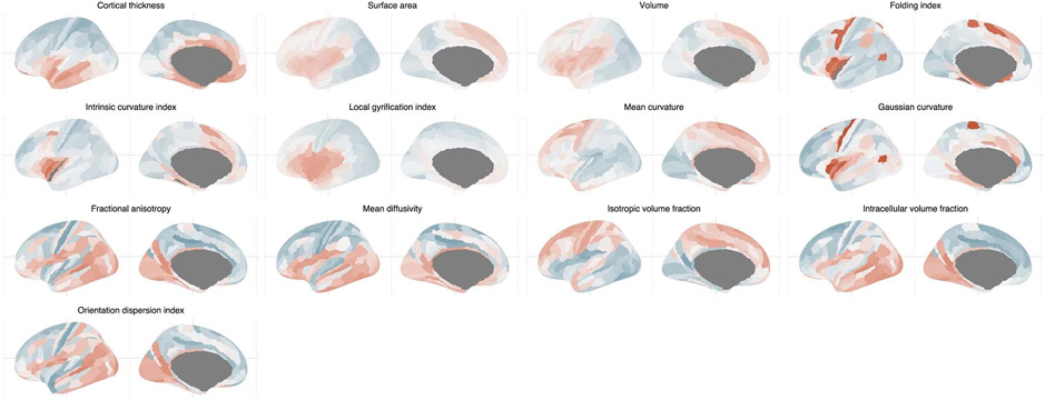
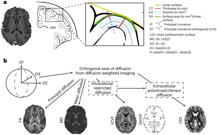
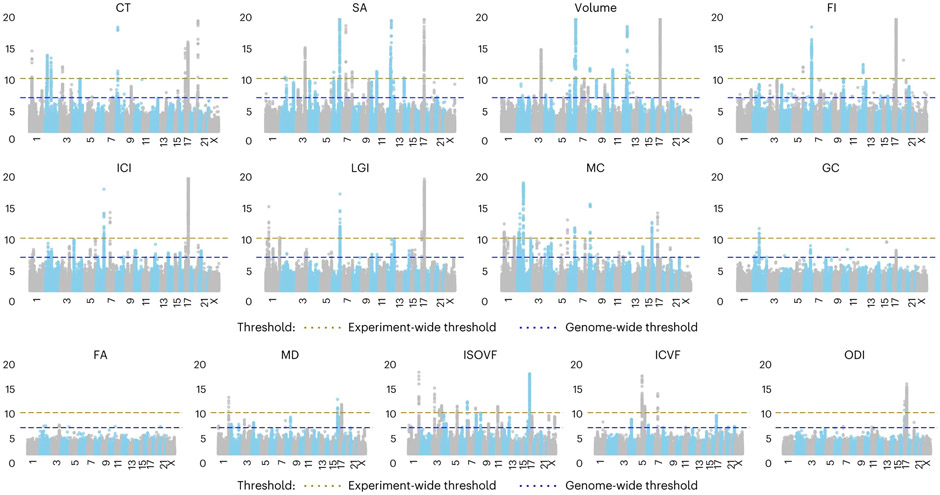
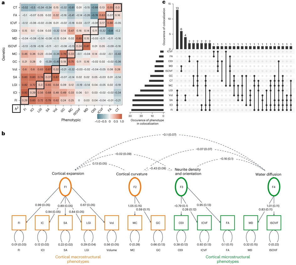
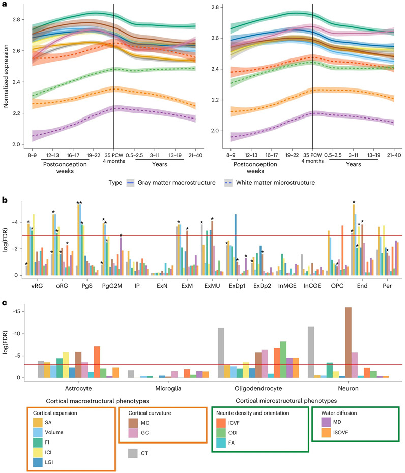
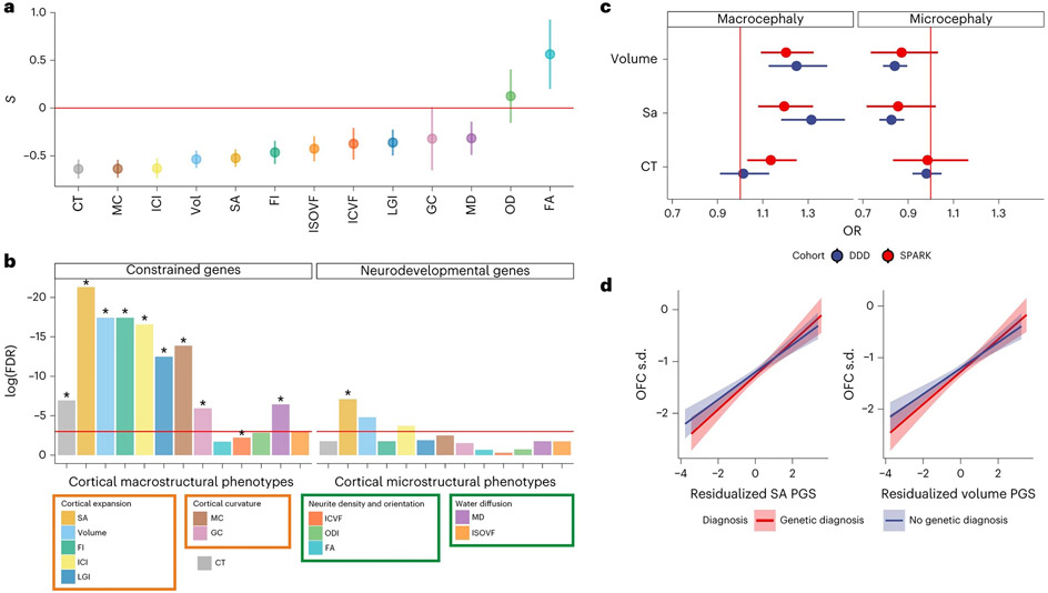
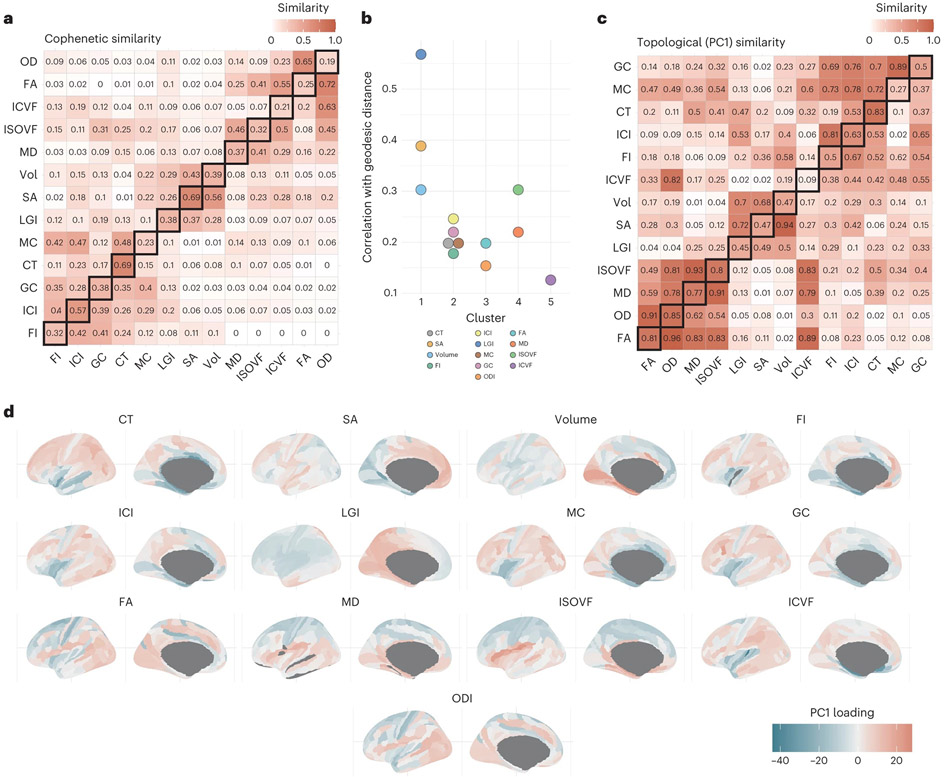
Our understanding of the genetics of the human cerebral cortex is limited both in terms of the diversity and the anatomical granularity of brain structural phenotypes. Here we conducted a genome-wide association meta-analysis of 13 structural and diffusion magnetic resonance imaging-derived cortical phenotypes, measured globally and at 180 bilaterally averaged regions in 36,663 individuals and identified 4,349 experiment-wide significant loci. These phenotypes include cortical thickness, surface area, gray matter volume, measures of folding, neurite density and water diffusion. We identified four genetic latent structures and causal relationships between surface area and some measures of cortical folding. These latent structures partly relate to different underlying gene expression trajectories during development and are enriched for different cell types. We also identified differential enrichment for neurodevelopmental and constrained genes and demonstrate that common genetic variants associated with cortical expansion are associated with cephalic disorders. Finally, we identified complex interphenotype and inter-regional genetic relationships among the 13 phenotypes, reflecting the developmental differences among them. Together, these analyses identify distinct genetic organizational principles of the cortex and their correlates with neurodevelopment.

Extended Data Fig. 1 ∣. Consistency in genetic effects between ABCD and UKB.

(a) Correlation in effect size (regression beta from GWAS) between ABCD and UKB cohorts for all 237 genome-wide significant SNPs in the UKB: Pearson’s correlation coefficient, r = 0.54 with 95% confidence interval 0.45–0.63. (b) Genetic correlation (central point) and 95% confidence intervals (error bars) for 12 global phenotypes in the UKB and ABCD cohorts. Given the relatively small size of ABCD, the intercept has been constrained as there is no participant overlap between the UKB (Nmax = 31,797) and ABCD (Nmax = 4,866) and there is no inflation in test statistics due to uncontrolled population stratification. Consequently, estimates of genetic correlation can be above 1.

Extended Data Fig. 2 ∣. Mendelian randomization analysis for causal relationships between genetic effects on global brain phenotypes.

Scatter plots for the bidirectional MR effects between surface area and folding index, intrinsic curvature index, and local gyrification index. Slopes of the line (MR regression coefficient) indicate the estimated MR effect by method. Linear a, b, and c are scatter plots where surface area is the exposure, and d, e, and f are scatter plots where surface area is the outcome. All scatter plots are for MR analyses conducted by splitting the UKB into two samples of similar sample sizes. All estimates were statistically significant in scatter plots A,B, and C. Inverse-variance weighted MR failed to reach statistical significance in scatter plots d, e, and f. Number of SNPs included in the MR are provided in Supplementary Table 9. Error bars represent standard errors of the effect size (point estimates).

Extended Data Fig. 3 ∣. Forest plots and leave-one-out plots.

Forest plots (a–c) and leave-one-out (d–f) between surface area and folding index (FI, A and D), Intrinsic curvature index (ICI, B and E), and local gyrification index (LGI, C and F). Number of SNPs included in the MR are provided in Supplementary Table 9. Error bars indicate 95% confidence intervals of the effect (point estimates).

Extended Data Fig. 4 ∣. Regional heritability.

a. The distribution of the SNP heritability for the 180 bilaterally-averaged regional phenotypes of the 13 neuroimaging modalities. Maximum GWAS sample size = 36,663. Box plots indicate the median value (central line), the interquartile range, and the whiskers indicate the minimum and maximum. b. The cortical spatial topology of SNP heritability for the 13 neuroimaging modalities.

Extended Data Fig. 5 ∣. Asymmetry indices and SNP heritability of asymmetry indices for the 13 phenotypes.

a. Asymmetry indices for the 13 phenotypes. Positive values indicate leftward asymmetry. b. SNP heritabilities for asymmetry indices by region and phenotype. SNP heritability was calculated using GCTA–GREML for approximately 9,650 unrelated individuals from the UK Biobank. Significant regions were identified after FDR correction within each of the 13 phenotypes.

Extended Data Fig. 6 ∣. Topography of the first phenotypic principal components.

Color scales depict the relative eigenvector ranging from −20 to +29, in all plots the midpoint is defined as 0. It should be noted that the sign is somewhat ambiguous and that the magnitude is relative to its own scaling (in this case within each phenotype for which the PCA is performed). Thus, in this context, the color scale indicates to what extent regions show more homogenous similarity (that is, regions with more similar color have more similar covariance).

Fig. 1 ∣. Schematic overview of 13 brain MRI phenotypes and the genetic analyses.

a, We considered eight cortical macrostructural phenotypes: CT, cortical SA, please note that this is for illustrative purposes and that the SA is measured at midthickness, gray matter volume (Vol), FI, ICI, LGI, MC and GC. b, We also considered five cortical microstructural phenotypes: FA, MD, ICVF (also called neurite density index (NDI)), ISOVF and ODI. Each phenotype was measured globally (total or mean for the whole cortex) and regionally at each of 180 bilaterally averaged cortical regions defined by the Human Connectome Project parcellation scheme. We conducted genome-wide association studies of all phenotypes after removing outliers and investigated the latent structure of all phenotypes, developmental trajectories and cell type specificity and genetic organization.

Fig. 2 ∣. Manhattan plots of GWAS meta-analysis of 13 global MRI phenotypes.

Blue dotted line indicates the threshold for genome-wide significance (P = 5 × 10⁻⁸), and the brown dotted line indicates the threshold for experiment-wide significance (P = 4.58 × 10⁻¹¹). Each dot on the x axis indicates an SNP and the y axis indicates the −log₁₀(P values). All analyses were conducted by linear mixed models.

Fig. 3 ∣. Pleiotropy among the 13 global phenotypes demonstrated by genetic/phenotypic correlations, structural equation modeling and colocalization analysis.

a, Phenotypic and genetic correlation matrices. The upper matrix triangle shows bivariate genetic correlations for each pair of phenotypes estimated using LDSC, and the lower triangle shows the pairwise phenotypic correlations (Spearman’s coefficient). The diagonal indicates the SNP heritability of each phenotype based on LDSC. Phenotypes are ordered based on hierarchical clustering of the genetic bivariate correlation (hierarchical clustering on the phenotypic correlation matrix resulted in a near identical ordering). b, Genomic SEM path diagram demonstrating the underlying latent structure of 12 of the 13 global phenotypes and the interfactor genetic correlations. Dashed lines connecting two variables, covariance relationships; double-headed arrows connecting a variable to itself, variance estimates; single-headed arrows pointing from independent variables to dependent variables, regression relationships. Circles indicate latent variables, and squares indicate measured phenotypes. The model was identified using unit variance identification such that the variance of the latent factors was set to one, and the dotted arrows across the factors can be interpreted as genetic correlation estimates. c, UpSet plot of the results of colocalization analysis demonstrating the numbers of genomic loci that colocalize between the 13 phenotypes. The dots correspond to the colocalized clusters, with the number of clusters in the vertical bars. The number of times a phenotype colocalizes is provided in the horizontal bars. Additionally, summary of clusters identified through GSEM and colocalization analyses and their relationship with other terms used in this study are also provided. Vol, gray matter volume.

Fig. 4 ∣. Enrichment of GWAS signals in different cell types during development.

a, Developmental trajectories of average gene expression in cortical postmortem-bulk RNA data (PsychEncode) for all significant genes (FDR < 0.05, n = 34–1,113; Supplementary Table 12) identified using H-MAGMA (left) or MAGMA (right) for 12 of the 13 global phenotypes. Data for FA are not shown as too few genes were identified as significant. The shaded region indicates 95% confidence intervals. b, Results of enrichment analyses for cell-specific gene expression from midgestation. FDR-corrected log₁₀(P values) for gene enrichment using genes identified from MAGMA (multiple regression) are plotted. The red line indicates the significance threshold at FDR-corrected P ≤ 0.05. Additionally, significant enrichments identified using H-MAGMA genes are indicated with an asterisk. c, Results of enrichment analyses from cell-specific epigenetic marks from postnatal cortex identified using LDSC-based enrichment. End, endothelial cells; ExDp1, excitatory deep layer neurons 1; ExDp2, excitatory deep layer neurons 2; ExM, maturing excitatory neurons; ExN, migrating excitatory neurons; ExMU, maturing excitatory neuron, upper enriched; InCGE, CGE interneuron; InMGE, MGE interneuron; IP, intermediate progenitors; OPC, oligodendrocyte precursor cells; oRG, outer radial glia; PgS and PgG2M, cycling progenitors, S phase and G2-M phase, respectively; Per, pericytes; vRG, ventral radial glia.

Fig. 5 ∣. Signatures of constraint and links to neurodevelopment for the global phenotypes.

a, Estimates of selection for the 13 cortical phenotypes. Selection coefficients (S), calculated with SBayesS, are provided as points on the y axis (points). Bars indicate 1 s.d. for the selection coefficients. Negative values indicate that lower-MAF alleles tend to have larger effect sizes. Sample sizes are sample sizes of the individual GWAS (n_max = 36,663). Vol, gray matter volume. b, Results of the enrichment analyses for constrained genes and genes associated with neurodevelopmental disorders using genes identified from MAGMA. FDR-corrected log₁₀(P values) for gene enrichment using genes identified from MAGMA (multiple regression) are shown (y axis). The red line indicates the significance threshold at FDR-adjusted P = 0.05. Additionally, significant enrichments identified using H-MAGMA genes are indicated with an asterisk c, Odds ratio (OR; provided as points) and 95% confidence intervals (error bars) for macrocephaly and microcephaly compared to individuals with neither for 1 s.d. increase in polygenic scores for volume, SA and CT in the DDD (n = 6,916) and SPARK (n = 25,621) cohorts. d, Line of best fit plotted using the linear model between genetic principal component corrected polygenic scores (SA and volume) and standardized (compared to the general population) occipital-frontal circumference (OFC s.d.) for individuals with or without a genetic diagnosis in the DDD cohort. The shaded region indicates 95% confidence intervals.

Fig. 6 ∣. Topographic similarity and principal component structure of cortical phenotypes.

a, Cophenetic similarity matrix depicting the similarity between the region × region similarity matrices. The upper triangle shows the cophenetic genetic similarity, the lower triangle shows the cophenetic phenotypic similarity and the diagonals show the phenotype–genotype cophenetic similarity across features. b, Correlation between network topology and geodesic distance organized by hierarchical clustering of the cophenetic similarity. c, Spatial correlation between the first principal component of each regional similarity matrix. The upper triangle shows the genetic similarity, the lower triangle shows the phenotypic similarity and the diagonals show the phenotype–genotype correlation across. d, Topology of the first genetic principal components, with color depicting the relative PCA eigenvalues. The color thus indicates to what extent regions show more homogenous similarity (that is, regions with more similar color have more similar covariance), but the actual sign and magnitude are relative within each phenotype.

References

1. Bethlehem RAI et al. Brain charts for the human lifespan. Nature 604, 525–533 (2022). - PMC - PubMed
1. Thompson PM et al. ENIGMA and global neuroscience: a decade of large-scale studies of the brain in health and disease across more than 40 countries. Transl. Psychiatry 10, 100 (2020). - PMC - PubMed
1. Gilmore JH, Knickmeyer RC & Gao W Imaging structural and functional brain development in early childhood. Nat. Rev. Neurosci 19, 123–137 (2018). - PMC - PubMed
1. Paus T, Keshavan M & Giedd JN Why do many psychiatric disorders emerge during adolescence? Nat. Rev. Neurosci 9, 947–957 (2008). - PMC - PubMed
1. Elliott LT et al. Genome-wide association studies of brain imaging phenotypes in UK Biobank. Nature 562, 210–216 (2018). - PMC - PubMed
Publication types