. 2023 Jul 21;4(8):100800.
doi: 10.1016/j.patter.2023.100800. eCollection 2023 Aug 11.

Understanding the host-pathogen evolutionary balance through Gaussian process modeling of SARS-CoV-2

Affiliations

Understanding the host-pathogen evolutionary balance through Gaussian process modeling of SARS-CoV-2

Salvatore Loguercio et al. Patterns (N Y). .

Abstract

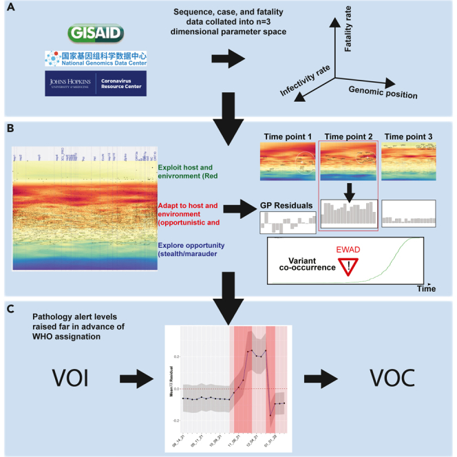
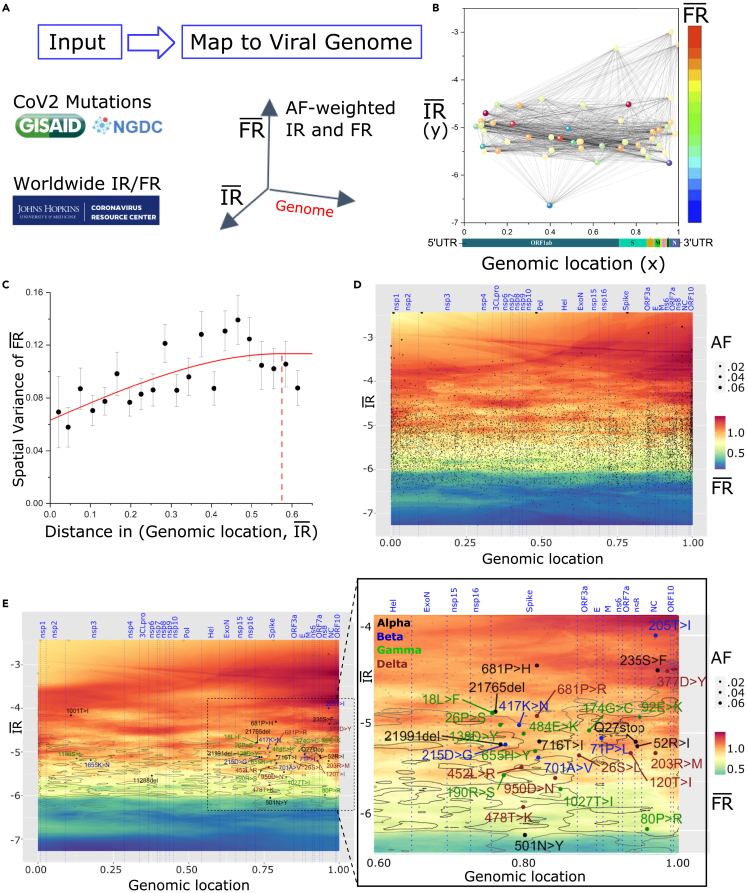
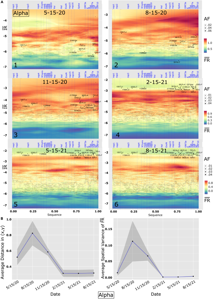
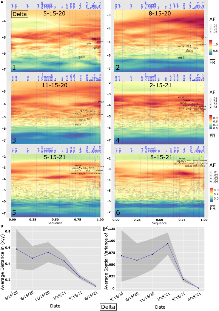
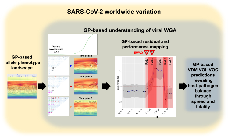
We have developed a machine learning (ML) approach using Gaussian process (GP)-based spatial covariance (SCV) to track the impact of spatial-temporal mutational events driving host-pathogen balance in biology. We show how SCV can be applied to understanding the response of evolving covariant relationships linking the variant pattern of virus spread to pathology for the entire SARS-CoV-2 genome on a daily basis. We show that GP-based SCV relationships in conjunction with genome-wide co-occurrence analysis provides an early warning anomaly detection (EWAD) system for the emergence of variants of concern (VOCs). EWAD can anticipate changes in the pattern of performance of spread and pathology weeks in advance, identifying signatures destined to become VOCs. GP-based analyses of variation across entire viral genomes can be used to monitor micro and macro features responsible for host-pathogen balance. The versatility of GP-based SCV defines starting point for understanding nature's evolutionary path to complexity through natural selection.

Keywords: Gaussian processes; SARS-CoV-2; early warning; evolution; genomic surveillance; host-pathogen; machine learning; spatial covariance.


Conflict of interest statement

The authors declare no competing interests. The authors declare no advisory, management or consulting positions. C.W. and W.E.B. have filed a patent application for the SCV methodology (serial no. US2021/0324474). C.W. and W.E.B. have filed a PCT application (serial no. PCT/US2022/039594) for VarC methodology.

Figures

None
Graphical abstract
Figure 1
Figure 1
Illustration of the GP regression approach (A) Data ingestion and pre-processing. Genotypic data from SARS-CoV-2 isolates and phenotypic data (cases and deaths) are gathered daily from NGDC and JH resource, respectively. For each reported SARS-CoV-2 mutation, allele frequency-weighted IR¯ and FR¯ are computed. (B) SARS-CoV-2 mutations (alleles) are positioned by their genomic positions (x axis) and IR¯ (y axis) and colored by FR¯ (z axis). The pairwise spatial relationships (indicated by black lines) are analyzed by GP regression. Shown is a simplified plot showing only 50 mutations for clarity. (C) As a first step in GP regression modeling, a variogram is computed (an illustrative example is depicted) showing spatial relationships between the separation distance of paired data points in (B) (x axis) and the spatial variance of FR¯ relative to IR¯ (y axis). (D and E) GP regression maps of genomic position (x axis), and log-transformed IR¯ (y axis) and FR¯ (color scale, z axis) for SARS-CoV-2 genome (data in this example are for 9/15/20). FR¯ is predicted across the whole landscape according to the variogram computed in (C), where output is an average of surrounding sample points, weighted by a function of distance given by the variogram. (D) Black dots represent variant input values used to compute GP regression, with dot sizes proportional to the allele frequency of the mutations. Vertical dotted blue lines are boundaries between SARS-CoV-2 proteins, annotated on the top axis. (E) Input variants are shaded light gray for clarity of VOCs. Contour lines are drawn at 10% and 25% percentiles of global variance estimated for model predictions (C). Labels on the map are signature mutations for Alpha (black), Beta (blue), Gamma (green), and Delta (brown). The zoomed inset shows the region with most VOC mutations in more detail, with all input mutations and contours that are used to train the GP regression model.
Figure 2
Figure 2
Time lapse of viral genome allele phenotype landscapes (A) Alpha VOC showing six tri-monthly time points between May 2020 and August 2021. IR¯ (y axis) and FR¯ (z axis) are log-transformed, genomic position is scaled to a (0–1) scaled from 5′ to 3′ of the RNA sequence encompassing ∼30,000 bp with 5′-end located at the origin of the x axis. Vertical dotted blue lines are boundaries between SARS-CoV-2 proteins, annotated on the top of each figure. Input variants are in shaded color, with dot sizes proportional to allele frequency of the mutations. Contour lines are drawn at 10% and 25% percentile of global variance estimated for model predictions (Figure 1C). (B and C) (Left) Average distance between Alpha VOC signature mutations defined by x axis (genomic position) and y axis coordinates (IR¯) as described in Figure 1B for each of the six time points shown in (A). The gray ribbon marks the 95% confidence interval. (Right) Average spatial variance of FR¯ (z axis) between Alpha signature mutations defined by x axis ‘Genome position’ and y axis coordinates (IR¯) as described in Figure 1B for each of the six time points shown in (C). The gray ribbon marks the 95% confidence interval.
Figure 3
Figure 3
Time lapse of viral genome allele phenotype landscapes (A) Delta VOC showing six tri-monthly time points between May 2020 and August 2021. IR¯ (y axis) and FR¯ (z axis) are log-transformed, genomic position is scaled to a (0–1) scaled from 5′ to 3′ of the RNA sequence encompassing ∼30,000 bp with 5′-end located at the origin of the x axis. Vertical dotted blue lines are boundaries between SARS-CoV-2 proteins, annotated on the top of each figure. Input variants are in shaded color, with dot sizes proportional to allele frequency of the mutations. Contour lines are drawn at 10% and 25% percentile of global variance estimated for model predictions (Figure 1C). (B) (Left) Average distance between Delta VOC signature mutations defined by x axis (genomic position) and y axis coordinates (IR¯) as described in Figure 1B for each of the six time points shown in (A). The gray ribbon marks the 95% confidence interval. (Right) Average spatial variance of FR¯ (z axis) between Delta signature mutations defined by x axis ‘Genome position’ and y axis coordinates (IR¯) as described in Figure 1B for each of the six time points shown in (A). The gray ribbon marks the 95% confidence interval.
Figure 4
Figure 4
Co-occurrence over time for VOCs (A) Timeline plots showing average cumulative co-occurrence (co-occurrence) over time for the four VOCs on the same scale (left), and zoom view on the later VOCs (Beta, Gamma, Delta). (B) Representative co-occurrence matrices showing co-occurrence counts between the signature mutations of each VOC. For both (A) and (B): Alpha VOC, black; Beta VOC, blue; Gamma VOC, green; Delta VOC, brown.
Figure 5
Figure 5
For each VOC (Alpha, Beta, Gamma, Delta), the upper panel reports min co-occurrence, max co-occurrence, average co-occurrence, and range (max co-occurrence minus min co-occurrence) between 9/15 and 8/22 The lower panel shows co-occurrence density, which is the number of non-zero co-occurrences over all possible co-occurrences, standardized for the range of 0–1, for the same time interval. To characterize more precisely co-occurrence patterns emerging for the four VOCs, we tracked max co-occurrence, min co-occurrence, and co-occurrence range over time instead of solely the average co-occurrence described above (upper panel of each). For Beta and Gamma, we observe a “high range” pattern where the difference between max and min co-occurrence (range co-occurrence: red line) increases over time and is above the curve for average co-occurrence (green line). Conversely, Alpha and Delta VOCs show a low range (red line) that is consistently below the average co-occurrence curve (green line) after co-occurrences begin accumulating at a steady pace. Beta and Gamma lineages are thought to boost the immune escape capabilities of the virus, while Alpha and Delta variants are more efficient in enhancing infectivity and spread. Thus, based on the detailed co-occurrence profiles, we can discriminate between different functional classes of VOCs.
Figure 6
Figure 6
EWAD analysis of Alpha, Beta, Gamma, and Delta VOCs (A) Graphical explanation of GP regression residuals. GP predictions are covariance-matrix weighted averages of the observed values, so a GP regression prediction is a point comprising the proximity weighted information of its surrounding observed values in the variant dark matter. The GP residual, calculated by using observed value minus the predicted value reports the difference between the mean observed FR¯ of that variant and the predicted FR¯—the weighted average of its surrounding variants. As illustrated, a positive GP residual indicates that the observed mean FR¯ of that variant is higher than the mean weighted averaging of the FR¯ for surrounding variants, while a negative GP residual indicates the predicted mean FR¯ of that variant is lower than the mean weighted averaging of the FR¯ for surrounding variants. GP residual values represent a real-time monitor for the differences of predicted variant FR¯ based on SCV analysis. (B–I) For each VOC (B and C, Alpha; D and E, Beta; F and G, Gamma; H and I, Delta), we report its average co-occurrence (co-occurrence plots: B, D, F, and H) together with the mean FR¯ residuals for its signature mutations (mean, blue line; 95% confidence interval, gray shade) computed weekly along the selected time interval (EWAD plots: C, E, G, and I). We examined the time interval between September 20 and May 21, and based on average co-occurrences, we selected six representative time points covering the flat, early, and sustained co-occurrence growth phases for each of the VOCs (see numbered points in graphs B–I). The baseline for EWAD is set to 0 ± 0.05 obtained by empirical randomization (dashed red line at 0 in EWAD plots) (C, E, G, and I) where for a VOC including n signature mutations, we computed the mean FR¯ residuals of thousands of random sets of n mutations yielding the interval near zero the random (null) EWAD signal. We then defined two alert levels, pathology alert level 1 (PAL1) (light red shades: C, E, G, and I) and pathology alert level 2 (PAL2) (dark red shades: C, E, G, and I) based on a heuristic that takes into account the degree of change over time, the magnitude of change, and the persistence over time where PAL1 includes two consecutive points whose combined change in mean FR¯ residual is above 0.05, and/or where both mean FR¯ residual and its 95% confidence interval are above/below zero. PAL2 includes three consecutive points whose combined change in mean FR¯ residual is above 0.1. Stars show the date that each variant was designated a VOC by the WHO.
Figure 7
Figure 7
Omicron VOC co-occurrence and EWAD spanning 8/15/21 to 3/20/22 (A) Time line plot showing average cumulative co-occurrence over time for combined Alpha, Beta, Gamma, and Omicron VOC defining mutations (Delta is out of range with values near 1M and is therefore omitted). (B) EWAD plot for combined Omicron where mean FR¯ residuals (blue line with 95% confidence interval, gray shade) for Omicron signature mutations computed weekly along the selected time intervals. The baseline for EWAD is set to 0 ± 0.05 by empirical randomization (dashed red line at 0; details as in Figure 6). Alert levels defined as in Figure 6. (C) Time line plot showing average cumulative co-occurrence over time for Omicron 1.1.529 and sub-lineages BA.1 and BA.2 for defining mutations. (D and E) Omicron sub-lineages BA.1 and BA.2 sub-lineages with co-occurrence over time and EWAD analysis between 1/17/22 and 3/20/22. EWAD plots for BA.1 and E. BA.2 where mean of FR¯ residuals (blue line; 95% confidence interval, gray shade) signature mutations computed weekly along the selected time interval. The baseline for EWAD is set to 0 ± 0.05 by empirical randomization (dashed red line at 0; details as in Figure 6). PAL defined as in Figure 6.
Figure 8
Figure 8
Flow diagram for modeling EWAD and performance using GP Starting from the GP-based predicted allele phenotype landscape for each VOC (leftmost panel) in combination with the co-occurrences at different time points (second panel from left), GP residuals can be calculated to assign PAL1 and PAL2 danger alerts (third panel from left) predicting the host-pathogen responses weeks to months ahead of the official WHO VOC assignation. The performance characteristics in terms of impact on VOC pandemic features can be estimated by the position of the mean FR¯ residuals below or above baseline (dotted line). Shown as an example is the result for Omicron emergence (Figure 7B).

Similar articles

Cited by

References

    1. WHO Coronavirus (COVID-19) Dashboard. (2022). https://covid19.who.int.
    1. Levin A.T., Hanage W.P., Owusu-Boaitey N., Cochran K.B., Walsh S.P., Meyerowitz-Katz G. Assessing the age specificity of infection fatality rates for COVID-19: systematic review, meta-analysis, and public policy implications. Eur. J. Epidemiol. 2020;35:1123–1138. doi: 10.1007/s10654-020-00698-1. - DOI - PMC - PubMed
    1. Channappanavar R., Perlman S. Age-related susceptibility to coronavirus infections: role of impaired and dysregulated host immunity. J. Clin. Invest. 2020;130:6204–6213. doi: 10.1172/JCI144115. - DOI - PMC - PubMed
    1. Niemi M.E.K., Karjalainen J., Liao R.G., Neale B.M., Daly M., Ganna A., Pathak G.A., Andrews S.J., Kanai M., Veerapen K., et al. Mapping the human genetic architecture of COVID-19. Nature. 2021;600:472–477. doi: 10.1038/s41586-021-03767-x. - DOI - PMC - PubMed
    1. Mendiola-Pastrana I.R., López-Ortiz E., Río de la Loza-Zamora J.G., González J., Gómez-García A., López-Ortiz G. SARS-CoV-2 Variants and Clinical Outcomes: A Systematic Review. Life. 2022;12 doi: 10.3390/life12020170. - DOI - PMC - PubMed

LinkOut - more resources