Recent parallel speciation in Antirrhinum involved complex haplotypes and multiple adaptive characters

Abstract

A role of ecological adaptation in speciation can be obscured by stochastic processes and differences that species accumulate after genetic isolation. One way to identify adaptive characters and their underlying genes is to study cases of speciation involving parallel adaptations. Recently resolved phylogenies reveal that alpine morphology has evolved in parallel in the genus Antirrhinum (snapdragons): first in an early split of an alpine from a lowland lineage and, more recently, from within the lowland lineage to produce closely related sympatric species with contrasting alpine and lowland forms. Here, we find that two of these later diverged sympatric species are differentiated by only around 2% of nuclear loci. Though showing evidence of recent gene flow, the species remain distinct for a suite of morphological characters typical of earlier-diverged alpine or lowland lineages and their morphologies correlate with features of the local landscape, as expected of ecological adaptations. Morphological differences between the two species involve multiple, unlinked genes so that parental character combinations are readily broken up by recombination in hybrids. We detect little evidence for post-pollination barriers to gene flow or recombination, suggesting that genetic isolation related to ecological adaptation is important in maintaining character combinations and might have contributed to parallel speciation. We also find evidence that genes involved in the earlier alpine-lowland split were reused in parallel evolution of alpine species, consistent with introgressive hybridisation, and speculate that many non-ecological barriers to gene flow might have been purged during the process.

Keywords: Antirrhinum; RADseq; adaptation; gene flow; introgression; snapdragon; speciation.

FIGURE 1

Parallel evolution of alpine morphology and A. barrelieri and A. rupestre phenotypes. (a) A cladogram showing assumed relationships between Antirrhinum species, based on Duran‐Castillo et al. (2021). Species with alpine morphology (taxonomic section Kickxiella) are in blue and taxonomic section Antirrhinum with lowland morphology in red. The two species in orange correspond to section Streptosepalum and are suggested to have evolved lowland morphology in parallel to the other lowland species. Where two species are unresolved they are shown on the same leaf. Supported nodes are marked with dots. (b) A representative of A. barrelieri (lowland morphology) in the field and (c–e) its glasshouse‐grown progeny. (f) A. rupestre (alpine morphology) in the field and (g–i) its glasshouse‐grown progeny. The same 150 mm ruler is shown in (b) and (f). Scale bars are 20 mm in (c) and (g) and 10 mm in (d, e) and (h, i).

FIGURE 2

Genetic differentiation of local Antirrhinum species. (a) The proportions of each individual's genome that was assigned to each of two (K = 2) or five (K = 5) ancestral populations are shown. Individuals are grouped according to location and the contribution of each ancestral haplotype is shown in a different colour along the y‐axis. (b) Locations of sampled A. barrelieri and A. rupestre populations are indicated with pie‐charts showing the mean genetic composition of each population, coloured as for K = 5 in (a). (c) Assignment at K = 2, as in (a), using all 506 loci, only the 11 loci with most biased distribution of alleles between A. barrelieri and A. rupestre, or the remaining 495 unbiased loci. (d) The average proportion of admixture in A. barrelieri and A. rupestre populations at K = 2, as in (a), plotted against minimum distance to a population of the other species. The p‐value is for no linear relationship. In contrast, admixture is not related to distance to the nearest population of the same species, as shown in the two panels to the right.

FIGURE 3

Morphological variation within A. rupestre and A. barrelieri correlates with genetics and habitat. (a) Principal components analysis of morphological variation in A. barrelieri and A. rupestre populations (each point represents the mean for one population). (b) Correlation between morphology of populations in the field and their progeny in a glasshouse (mean population morphology indices ±1 SD; b A. barrelieri, r A. rupestre). (c) The relationship of intermediate morphology to proximity of the other species. Intermediate morphology is the difference between the morphology index of each population and the most extreme value for the species. Distance is the distance of each population to the nearest population of the other species. (d) Association of morphology and genetics with different features of habitat represented as the first two dimensions of a canonical correspondence analysis (CCA). Categories used for each variable are detailed in Section 2. All associations are significant with p ≤ .04. (e) Morphology index plotted against genetic index (the proportion of the genome assigned to A. rupestre in Structure analysis at K = 2). ‘Training’ plants were the least genetically admixed individuals used to derive the morphology index. p = 2 × 10⁻³⁴ and R = .84 for all individuals, and p = 6.0 × 10⁻¹² and R = .69 with training plants excluded (the regression line is the same for both). (f) Morphological variation in F₁ and F₂ hybrids of A. rupestre × A. barrelieri compared to allopatric representatives of the parent species. Samples sizes are given in Section 2 and in Table S1.

FIGURE 4

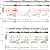
Polymorphism and linkage in A. barrelieri and A. rupestre genomes. (a) Gene density plotted along a physical map of the A. majus genome. Coordinates are in Mbp. (b) Sliding‐window plots of the predicted density of Sbf I sites (light grey) and RADseq loci recovered from both A. barrelieri and A. rupestre (black)—sequences unique to one species were not included. (c) Physical locations of polymorphic RADseq loci that were homozygous in both parents (2), one parent (1) or neither (0). (d) A linkage map of RADseq loci. Slanted lines compare the map position of each marker with its physical position in the A. majus genome. (e) Proportions of genotypes in the F₂ population compared to the expected proportions of 0.5 for heterozygotes and 0.25 for each homozygote in the absence of distorted transmission (r = A. rupestre, b = A. barrelieri). The proportion of alleles from A. barrelieri is plotted separately for the region of Chr1 showing distorted genotype ratios.

FIGURE 5

QTL underlying morphological differences between A. barrelieri and A. rupestre. The most likely position of each significant QTL is shown by an arrow with a length proportional to the magnitude of the QTL effect and an orientation reflecting the direction of parental alleles (upwards pointing shows that the A. barrelieri allele increase the character value). Estimates of 0.95 and 0.99 confidence intervals for QTL positions are shown by thick and thin horizontal lines, respectively. The position at which the line cuts the arrow represents the relative trait value estimated for heterozygotes (e.g. the A. barrelieri allele at locus LfLW5 is fully dominant). The percentage of F₂ variance explained (PVE) is given for loci individually and in total. No significant QTL was detected for the remaining traits. The positions of markers used in QTL analysis are shown on the linkage map above the positions of the QTL.

References

1. Antao, T. , & Beaumont, M. A. (2011). Mcheza: A workbench to detect selection using dominant markers. Bioinformatics, 27(12), 1717–1718. 10.1093/bioinformatics/btr253 - DOI - PubMed
1. Arendt, J. , & Reznick, D. (2008). Convergence and parallelism reconsidered: What have we learned about the genetics of adaptation? Trends in Ecology & Evolution, 23(1), 26–32. 10.1016/j.tree.2007.09.011 - DOI - PubMed
1. Barton, N. H. , & De Cara, M. A. R. (2009). The evolution of strong reproductive isolation. Evolution, 63(5), 1171–1190. 10.1111/j.1558-5646.2009.00622.x - DOI - PubMed
1. Bertel, C. , Rešetnik, I. , Frajman, B. , Erschbamer, B. , Hülber, K. , & Schönswetter, P. (2018). Natural selection drives parallel divergence in the mountain plant Heliosperma pusillum s.l. Oikos, 127(9), 1355–1367. 10.1111/oik.05364 - DOI
1. Billings, W. D. (1974). Adaptations and origins of alpine plants. Arctic and Alpine Research, 6(2), 129–142. 10.1080/00040851.1974.12003769 - DOI
Publication types
LinkOut - more resources