Within-Individual Organization of the Human Cerebral Cortex: Networks, Global Topography, and Function

Abstract

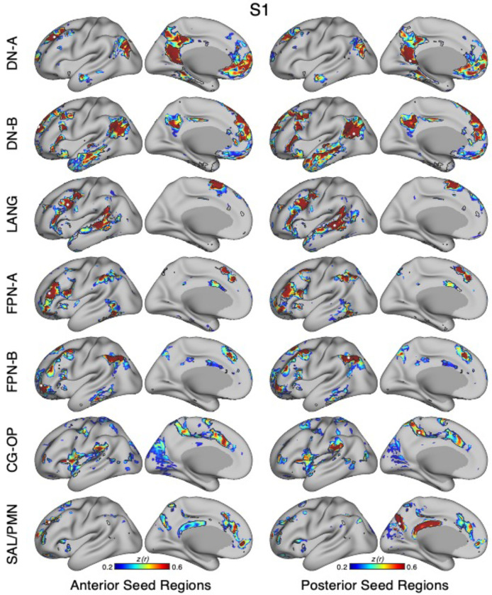
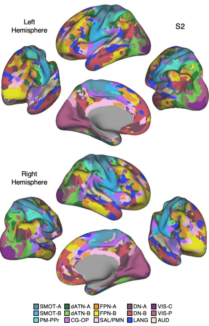
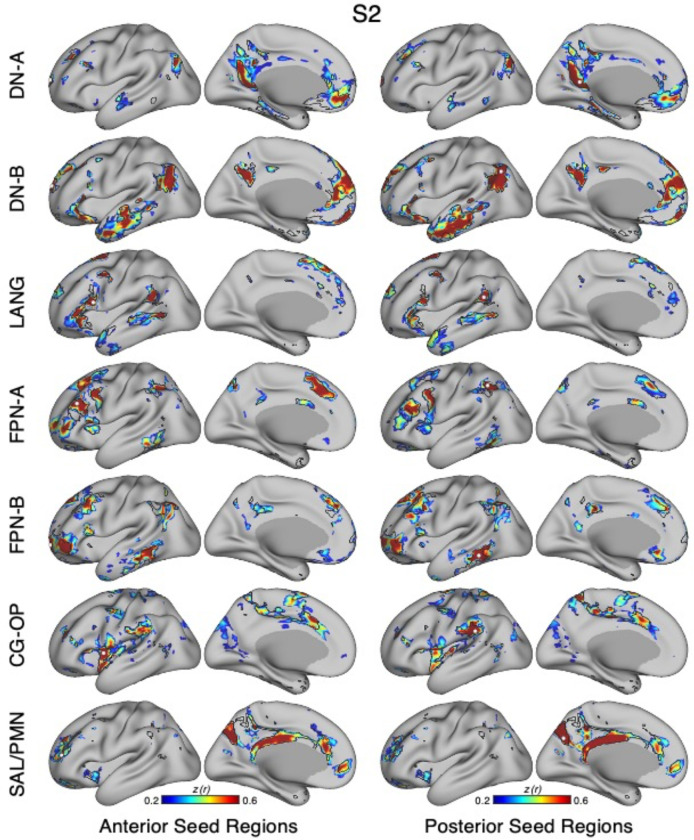
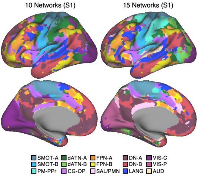
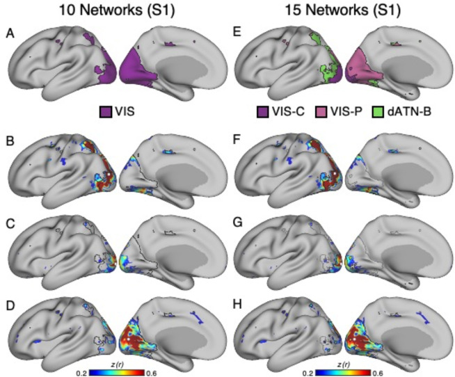
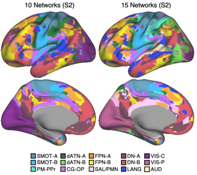
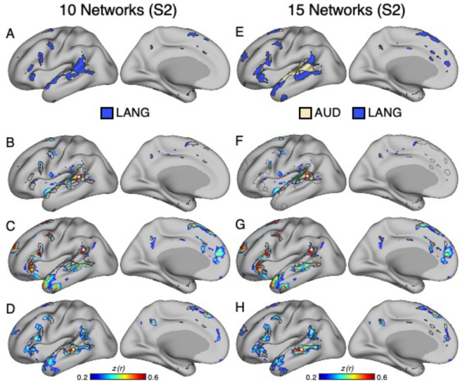
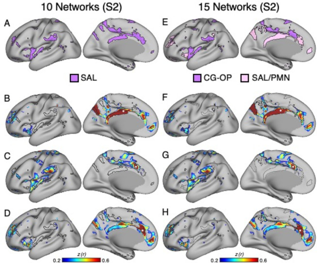
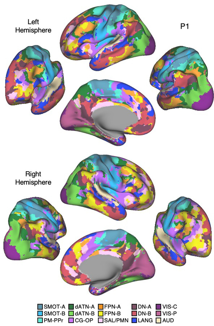
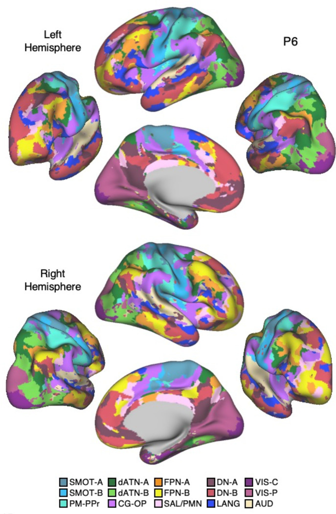
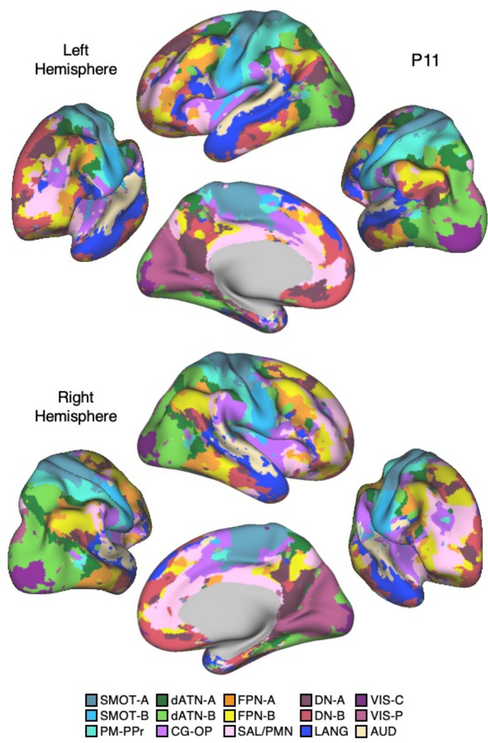
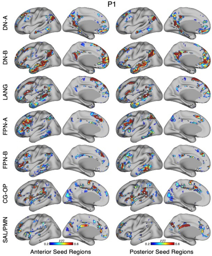
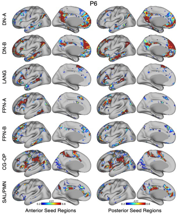
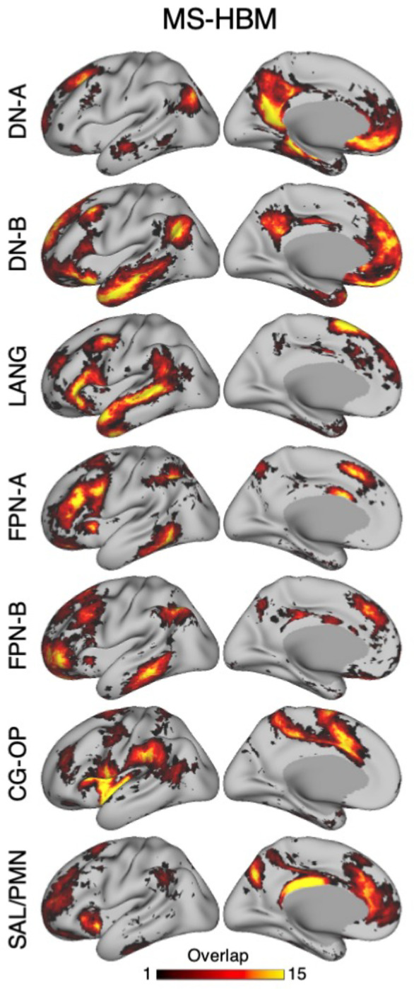
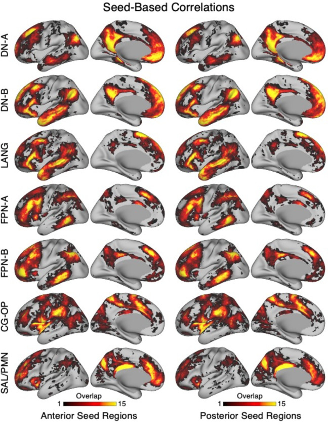
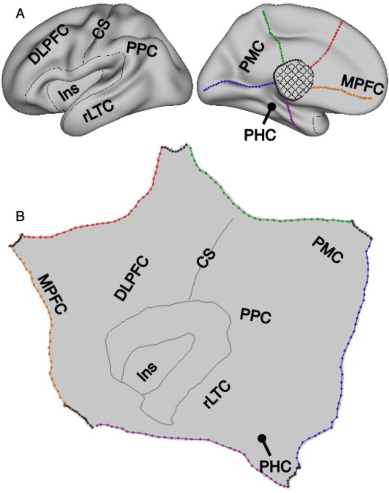
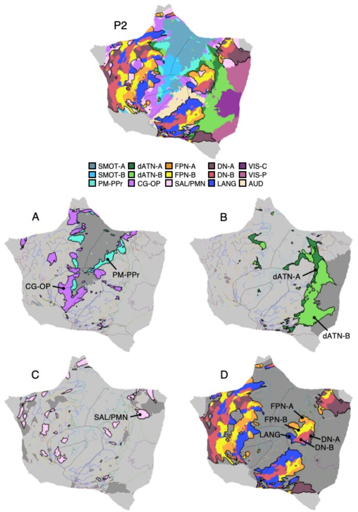
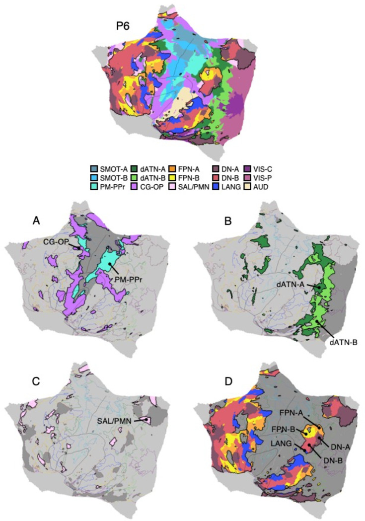
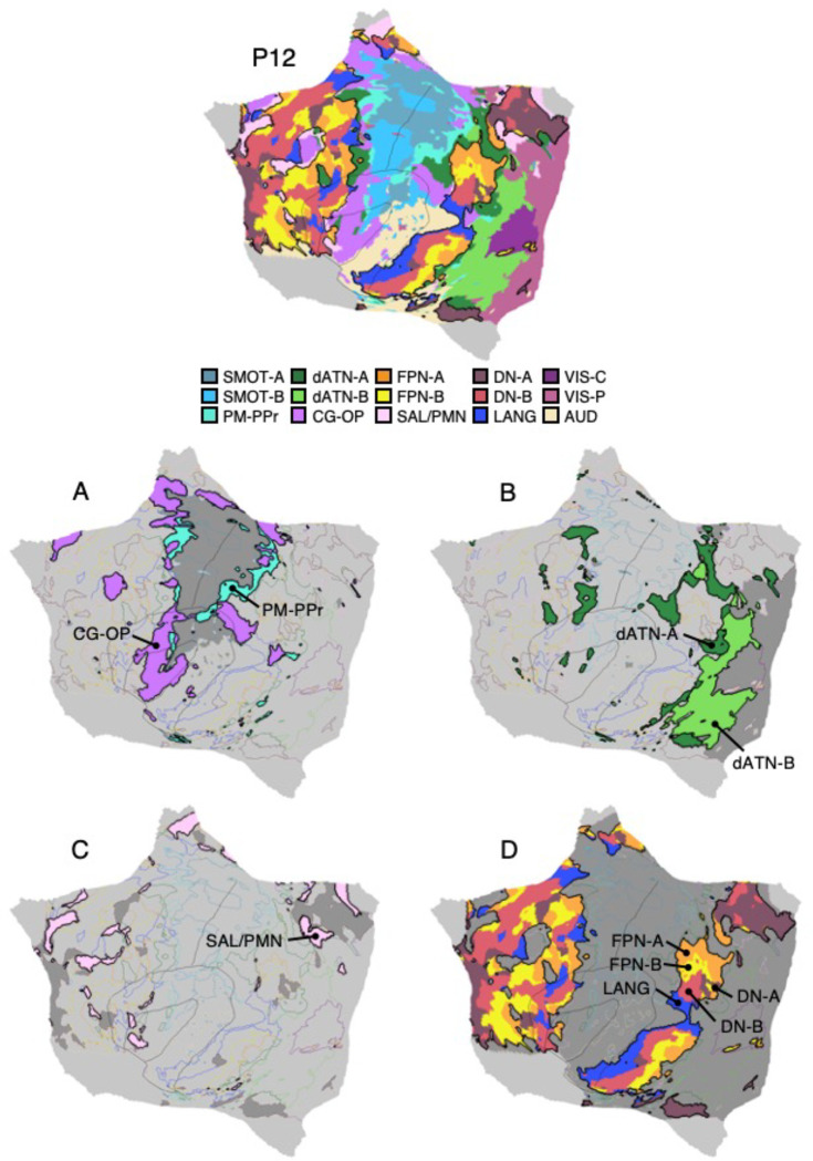
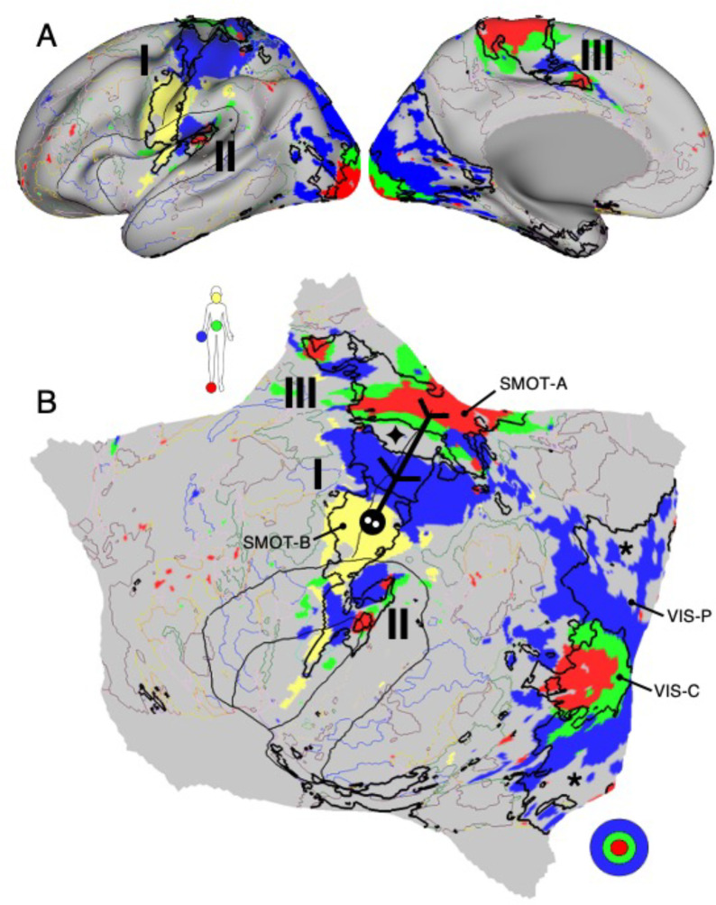
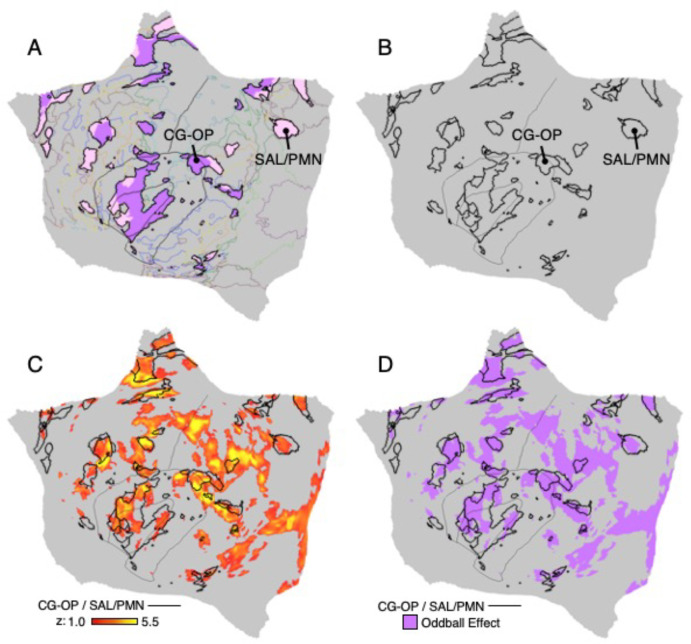
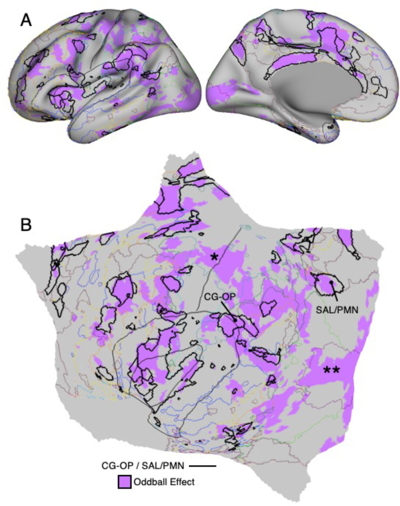
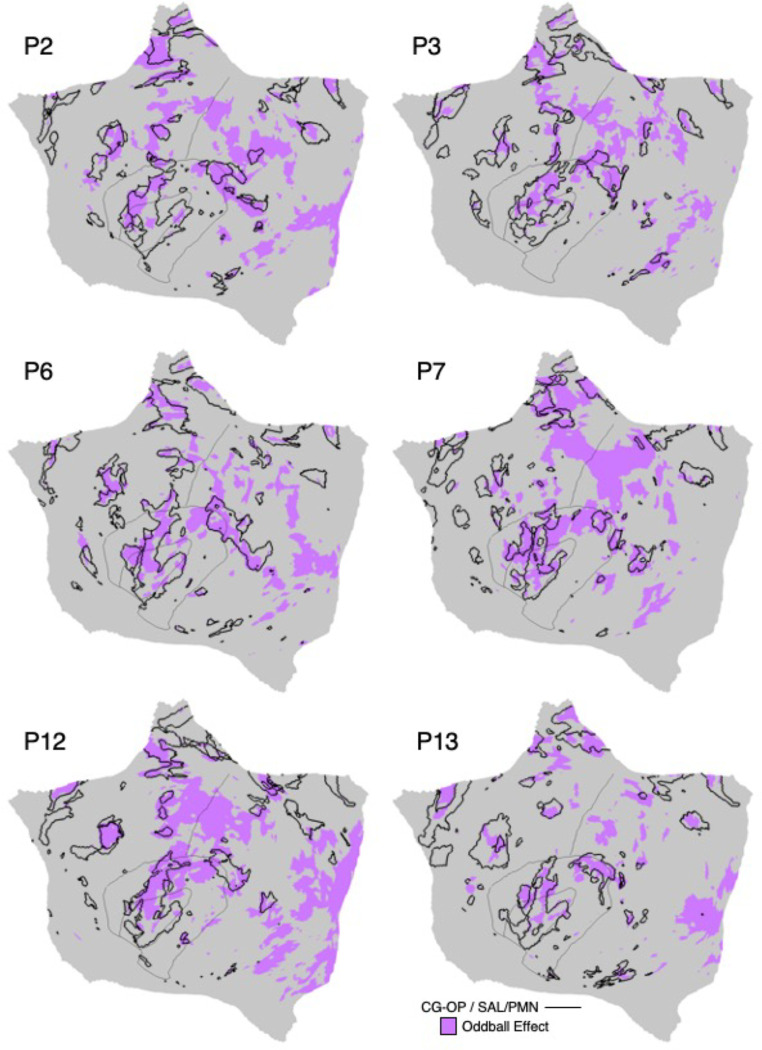
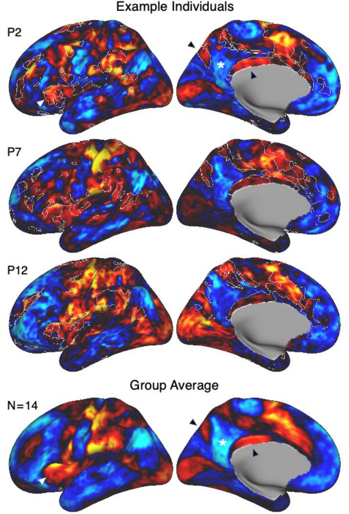
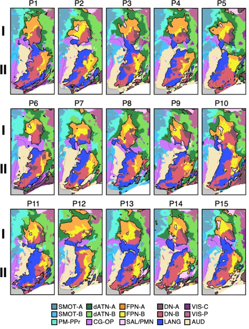
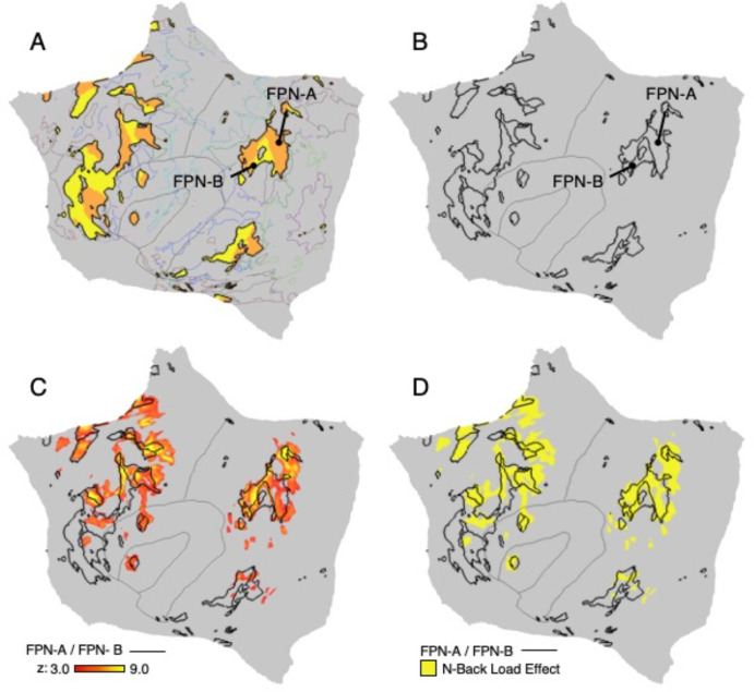
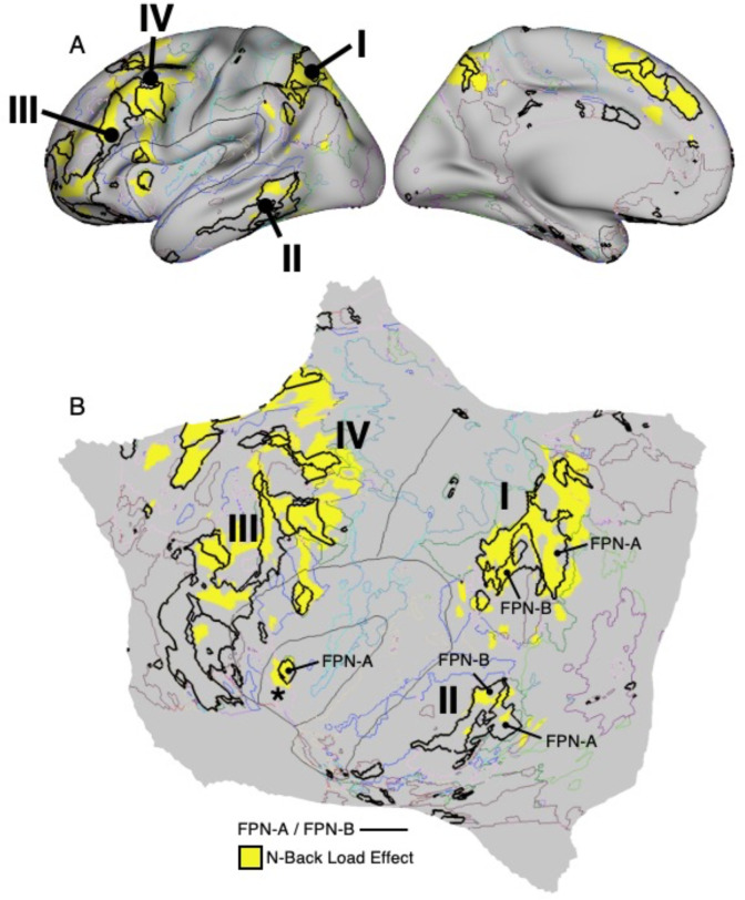
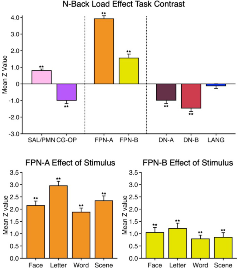
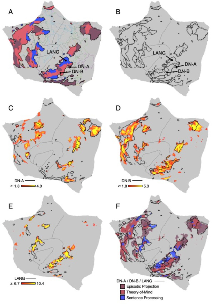
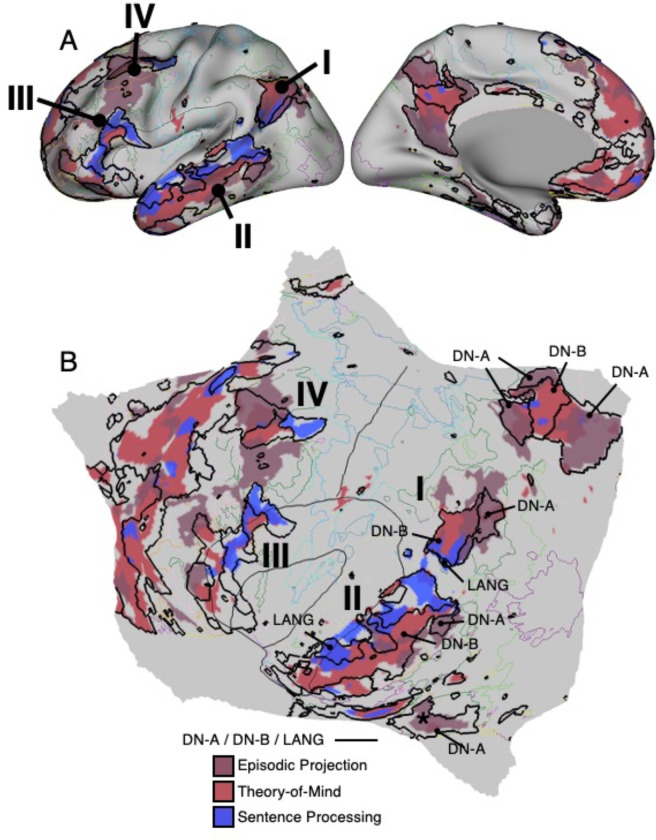
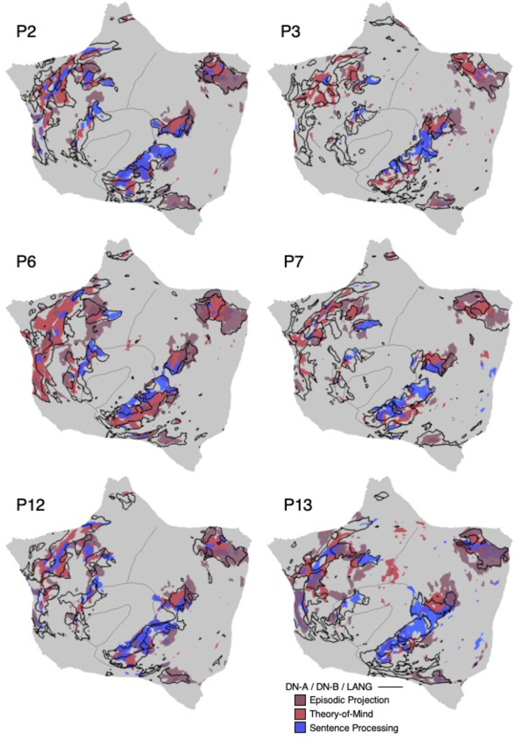
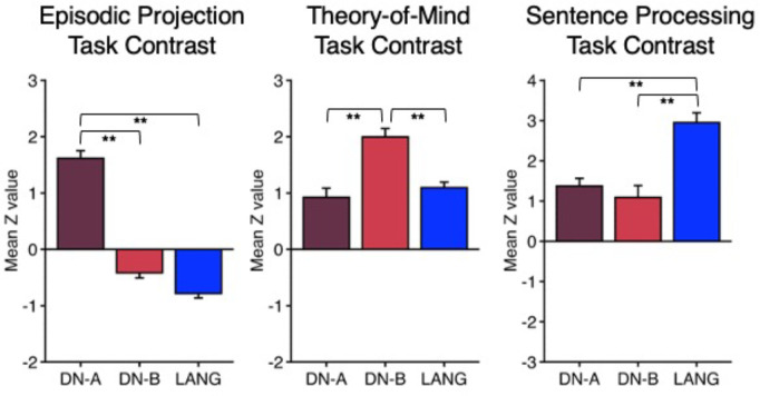
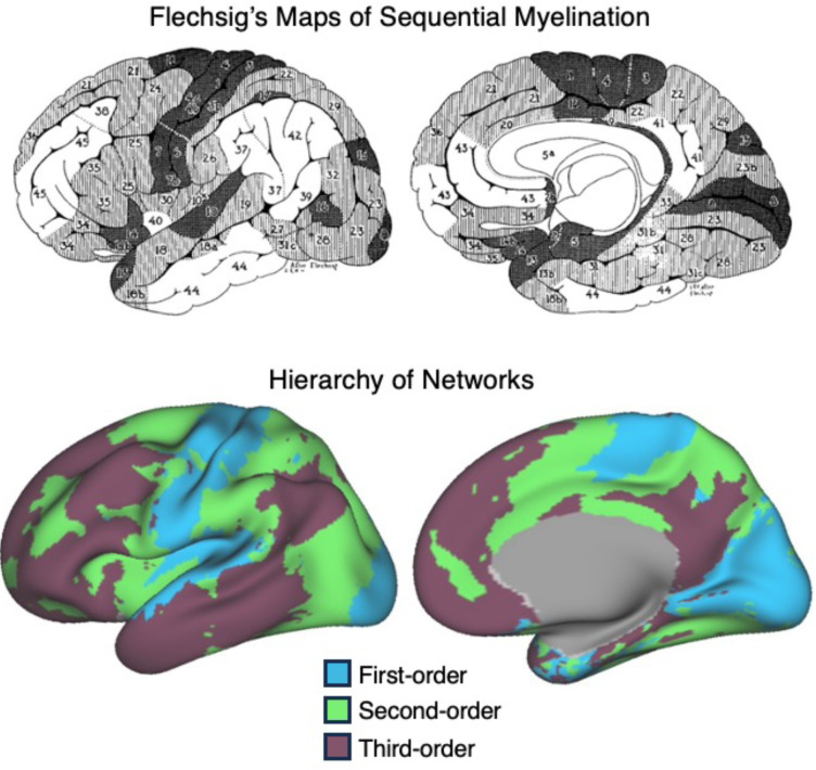
The human cerebral cortex is populated by specialized regions that are organized into networks. Here we estimated networks using a Multi-Session Hierarchical Bayesian Model (MS-HBM) applied to intensively sampled within-individual functional MRI (fMRI) data. The network estimation procedure was initially developed and tested in two participants (each scanned 31 times) and then prospectively applied to 15 new participants (each scanned 8 to 11 times). Detailed analysis of the networks revealed a global organization. Locally organized first-order sensory and motor networks were surrounded by spatially adjacent second-order networks that also linked to distant regions. Third-order networks each possessed regions distributed widely throughout association cortex. Moreover, regions of distinct third-order networks displayed side-by-side juxtapositions with a pattern that repeated similarly across multiple cortical zones. We refer to these as Supra-Areal Association Megaclusters (SAAMs). Within each SAAM, two candidate control regions were typically adjacent to three separate domain-specialized regions. Independent task data were analyzed to explore functional response properties. The somatomotor and visual first-order networks responded to body movements and visual stimulation, respectively. A subset of the second-order networks responded to transients in an oddball detection task, consistent with a role in orienting to salient or novel events. The third-order networks, including distinct regions within each SAAM, showed two levels of functional specialization. Regions linked to candidate control networks responded to working memory load across multiple stimulus domains. The remaining regions within each SAAM did not track working memory load but rather dissociated across language, social, and spatial / episodic processing domains. These results support a model of the cerebral cortex in which progressively higher-order networks nest outwards from primary sensory and motor cortices. Within the apex zones of association cortex there is specialization of large-scale networks that divides domain-flexible from domain-specialized regions repeatedly across parietal, temporal, and prefrontal cortices. We discuss implications of these findings including how repeating organizational motifs may emerge during development.

Figure 1.. Temporal signal-to-noise ratio (SNR) map for S1.

The mean estimate of temporal SNR for the fMRI data is illustrated for multiple views of the left hemisphere on the inflated cortical surface (from 62 runs collected over 31 days). Note the low SNR within the orbitofrontal cortex and the temporal pole. This pattern is typical of the data across all participants in the present work and should be considered when evaluating network organization. A, anterior; P, posterior; D, dorsal; V, ventral. SNR maps for all participants are provided in the Supplementary Materials.

Figure 2.. 15-network cerebral cortical parcellation estimated for S1.

Network estimates from the multi-session hierarchical Bayesian model (MS-HBM) are displayed across four views. The left hemisphere is on top and right hemisphere below. Each color represents a distinct network estimated by the model. Some networks possess primarily local organization (e.g., Somatomotor, Visual), while other networks possess widely distributed organization (e.g., those involving prefrontal, temporal, and parietal association zones). The network labels are used similarly throughout the figures. SMOT-A, Somatomotor-A; SMOT-B, Somatomotor-B; PM-PPr, Premotor-Posterior Parietal Rostral; CG-OP, Cingular-Opercular; SAL / PMN, Salience / Parietal Memory Network; dATN-A, Dorsal Attention-A; dATN-B, Dorsal Attention-B; FPN-A, Frontoparietal Network-A; FPN-B, Frontoparietal Network-B; DN-A, Default Network-A; DN-B, Default Network-B; LANG, Language; VIS-C, Visual Central; VIS-P, Visual Peripheral; AUD, Auditory.

Figure 3.. Model-free confirmation of networks using seed-region correlation for S1.

The correlation patterns from individual seed regions placed within networks are displayed. In each row, a distinct network is targeted, labeled to the left. The two left columns display correlation maps using an anterior seed region of each network, while the two right columns display correlation maps using a posterior seed region. Lateral and medial views are displayed. White-filled circles display the seed region locations. Black outlines show the boundaries of individual-specific networks estimated from the MS-HBM as shown in Fig. 2. The correlation maps are plotted as z(r) with the color scale at the bottom. The correlation maps are not constrained to fall within the estimated network boundaries. Nonetheless, the network boundaries capture a great deal of the spatial correlational properties of the underlying data.

Figure 4.. Temporal signal-to-noise ratio (SNR) map for S2.

Paralleling Fig. 1, the mean estimate of temporal SNR for the fMRI data is illustrated for multiple views of the left hemisphere on the inflated cortical surface (from 61 runs collected over 31 days). A, anterior; P, posterior; D, dorsal; V, ventral.

Figure 5.. 15-network cerebral cortical parcellation estimated for S2.

Paralleling Fig. 2, network estimates from the MS-HBM are displayed across four views. The left hemisphere is on top and right hemisphere below. Each color represents a distinct network estimated by the model. The names of cortical networks are shown at the bottom.

Figure 6.. Model-free confirmation of networks using seed-region correlation for S2.

Paralleling Fig. 3, the correlation patterns from individual seed regions placed within networks are displayed for S2. The two left columns display correlation maps using an anterior seed region for each network, while the two right columns display correlation maps using a posterior seed region. Lateral and medial views are displayed for each seed region. White-filled circles display the seed region locations. Black outlines indicate the boundaries of corresponding individual-specific parcellation-defined networks estimated from the MS-HBM as shown in Fig. 5. The correlation maps are plotted as z(r) with the color scale at the bottom.

Figure 7.. Direct comparison of 10-network and 15-network cerebral cortical parcellations for S1.

The left displays the 10-network estimate and the right the 15-network estimate. Many of the major networks are similar between the two parcellations, including LANG, DN-A, DN-B, FPN-A, FPN-B, SMOT-A, SMOT-B. VIS in the 10-network estimate is differentiated into dATN-B, VIS-C and VIS-P in the 15-network estimate. A monolithic large network in the 10-network estimate is differentiated into SAL / PMN and CG-OP in the 15-network estimate. dATN in the 10-network estimate is differentiated into dATN-A and PM-PPr in the 15-network estimate, and a distinct AUD network emerges near to LANG and SMOT-B. The network labels are shown at the bottom.

Figure 8.. Model-free estimates illustrate the utility of the 15-network cerebral parcellation for visual networks for S1.

Seed region correlation maps illustrate features captured by the 15-network estimate as contrast to the 10-network estimate. VIS in the 10-network estimate (A) is differentiated into dATN-B, VIS-C and VIS-P in the 15-network estimate (E). White-filled circles display the seed region locations. Black outlines indicate the boundaries of the networks above. The network labels are shown below. Correlation maps for three distinct seed regions in and around the vicinity of visual cortex are illustrated within the boundaries of the 10-network estimate (B, C, D) and the 15-network estimate (F, G, H). Note that the correlation patterns are well captured by the 15-network estimate. Black and gray outlines illustrate the networks from each parcellation estimate. The correlation maps are plotted as z(r) with the color scale at the bottom.

Figure 9.. Model-free estimates illustrate the utility of the 15-network cerebral parcellation for networks surrounding somatomotor cortex for S1.

Paralleling Fig. 8, seed region correlation maps illustrate features captured by the 15-network estimate as contrast to the 10-network estimate. dATN in the 10-network estimate (A) is differentiated into dATN-A and PM-PPr in the 15-network estimate (E). White-filled circles display the seed region locations. Black outlines indicate the boundaries of the networks above. The network labels are shown below. Correlation maps for three distinct seed regions surrounding somatomotor cortex are illustrated within the boundaries of the 10-network estimate (B, C, D) and the 15-network estimate (F, G, H). Black and gray outlines illustrate the networks from each parcellation estimate. The correlation maps are plotted as z(r) with the color scale at the bottom.

Figure 10.. Direct comparison of 10-network and 15-network cerebral cortical parcellations for S2.

Paralleling Fig. 7, the left displays the 10-network estimate and the right the 15-network estimate. The network labels are shown at the bottom.

Figure 11.. Model-free estimates illustrate the utility of the 15-network cerebral parcellation for auditory and language networks for S2.

Seed region correlation maps illustrate features captured by the 15-network estimate as contrast to the 10-network estimate. LANG in the 10-network estimate (A) is differentiated into AUD and LANG in the 15-network estimate (E). White-filled circles display the seed region locations. Black outlines indicate the boundaries of the networks above. The network labels are shown below. Correlation maps for three distinct seed regions in and around the vicinity of auditory cortex are illustrated within the boundaries of the 10-network estimate (B, C, D) and the 15-network estimate (F, G, H). Black and gray outlines illustrate the networks from each parcellation estimate. The correlation maps are plotted as z(r) with the color scale at the bottom.

Figure 12.. Model-free estimates illustrate the utility of the 15-network cerebral parcellation for networks at and around cingulate cortex for S2.

Paralleling Fig. 11, seed region maps illustrate features captured by the present 15-network estimate as contrast to the 10-network estimate. SAL in the 10-network estimate (A) is differentiated into the SAL / PMN and the CG-OP networks in the 15-network estimate (E). White-filled circles display the seed region locations. Black outlines indicate the boundaries of the networks above. The network labels are shown below. Correlation maps for three seed regions around the cingulate are illustrated within the boundaries of the 10-network estimate (B, C, D) and the 15-network estimate (F, G, H). Black and gray outlines illustrate the networks from each parcellation estimate. The correlation maps are plotted as z(r) with the color scale at the bottom.

Figure 13.. Cerebral cortical network estimates are reliable across independent datasets within individuals.

Independently analyzed subsets of data from S1 (Top) and S2 (Bottom) illustrate the reliability of the network estimates. The resting-state fixation data of S1 and S2 were split into three datasets to estimate networks using the MS-HBM applied independently to each dataset. The individual-specific cortical parcellations are replicable within participants, critically for models based on ~20 runs of resting-state fixation data as will be employed for the 15 new participants analyzed throughout the remainder of this paper. The network labels are shown at the bottom.

Figures 14–16.. Network estimates for novel participants.

Networks estimated for representative participants from the novel discovery (P1), replication (P6) and triplication (P11) datasets are displayed. The network estimates are from the 15-network MS-HBM. Four views for each hemisphere show details of cortical network organization, with lateral and medial views as well as rotated frontal and posterior views. The left hemisphere is on top and right hemisphere below. Each color represents a distinct network with the network labels shown at the bottom. Similar maps for all available participants are provided in the Supplementary Materials.

Figures 14–16.. Network estimates for novel participants.

Networks estimated for representative participants from the novel discovery (P1), replication (P6) and triplication (P11) datasets are displayed. The network estimates are from the 15-network MS-HBM. Four views for each hemisphere show details of cortical network organization, with lateral and medial views as well as rotated frontal and posterior views. The left hemisphere is on top and right hemisphere below. Each color represents a distinct network with the network labels shown at the bottom. Similar maps for all available participants are provided in the Supplementary Materials.

Figures 14–16.. Network estimates for novel participants.

Networks estimated for representative participants from the novel discovery (P1), replication (P6) and triplication (P11) datasets are displayed. The network estimates are from the 15-network MS-HBM. Four views for each hemisphere show details of cortical network organization, with lateral and medial views as well as rotated frontal and posterior views. The left hemisphere is on top and right hemisphere below. Each color represents a distinct network with the network labels shown at the bottom. Similar maps for all available participants are provided in the Supplementary Materials.

Figures 17–19.. Model-free confirmation of networks using seed-region based correlation for the implementation stage participants.

The correlation patterns from individual seed regions placed within networks are displayed for representative participants from the novel discovery (P1), replication (P6) and triplication (P11) datasets. The two left columns display correlation maps using an anterior seed region for each network, while the two right columns display correlation maps using a posterior seed region. Lateral and medial views are displayed for each seed region. Black outlines indicate the boundaries of corresponding individual-specific parcellation-defined networks estimated from the MS-HBM as shown in Figs. 14–16. The correlation maps are plotted as z(r) with the color scale at the bottom. Strong agreement is evident between the seed-region based correlation maps and the estimated network boundaries. Similar maps for all available participants are provided in the Supplementary Materials.

Figures 17–19.. Model-free confirmation of networks using seed-region based correlation for the implementation stage participants.

The correlation patterns from individual seed regions placed within networks are displayed for representative participants from the novel discovery (P1), replication (P6) and triplication (P11) datasets. The two left columns display correlation maps using an anterior seed region for each network, while the two right columns display correlation maps using a posterior seed region. Lateral and medial views are displayed for each seed region. Black outlines indicate the boundaries of corresponding individual-specific parcellation-defined networks estimated from the MS-HBM as shown in Figs. 14–16. The correlation maps are plotted as z(r) with the color scale at the bottom. Strong agreement is evident between the seed-region based correlation maps and the estimated network boundaries. Similar maps for all available participants are provided in the Supplementary Materials.

Figures 17–19.. Model-free confirmation of networks using seed-region based correlation for the implementation stage participants.

The correlation patterns from individual seed regions placed within networks are displayed for representative participants from the novel discovery (P1), replication (P6) and triplication (P11) datasets. The two left columns display correlation maps using an anterior seed region for each network, while the two right columns display correlation maps using a posterior seed region. Lateral and medial views are displayed for each seed region. Black outlines indicate the boundaries of corresponding individual-specific parcellation-defined networks estimated from the MS-HBM as shown in Figs. 14–16. The correlation maps are plotted as z(r) with the color scale at the bottom. Strong agreement is evident between the seed-region based correlation maps and the estimated network boundaries. Similar maps for all available participants are provided in the Supplementary Materials.

Figure 20.. Overlap of network estimates derived from the MS-HBM model.

Each row displays the overlap map from one target network for the full set of 15 novel participants using the estimates from the 15-network MS-HBM. The network targets are labeled to the left. DN-A, DN-B, LANG, FPN-A, FPN-B, CG-OP, and SAL / PMN networks are examined separately. The purpose of these maps is to illustrate the overlap of network organization across participants as well as illustrate how the separate networks are distinct from one another.

Figure 21.. Overlap of network estimates derived from model-free seed-region correlation maps.

Each row displays the overlap map from one target network for the full set of 15 novel participants using only seed-region based correlation estimates of the networks. In the left two columns, each row displays the overlap map of correlation patterns based on an anterior seed region. In the right two columns, each row displays the overlap map based on a posterior seed region. The network targets are labeled to the left. DN-A, DN-B, LANG, FPN-A, FPN-B, CG-OP, and SAL / PMN networks are examined separately. The purpose of these maps is to illustrate the overlap of network organization without strong model assumptions (priors) that might bias the degree of overlap.

Figure 22.. Visualization on the flattened cortical surface.

A fully flattened cortical surface was constructed to better reveal topographic relations among networks. By applying five cuts along the colorful lines on the midline, the inflated cortical surface (A) was flattened (B). The five cuts included one cut along the calcarine sulcus (blue dotted line) and four additional cuts radiating outwards from the medial wall. The surface enclosed by the circular cut was removed. Reference lines illustrate the inner and outer boundaries of the insula (Ins) as well as along the central sulcus (CS). Additional landmarks are dorsolateral PFC (DLPFC), posterior parietal cortex (PPC), rostral lateral temporal cortex (rLTC), posteromedial cortex (PMC), parahippocampal cortex (PHC), and medial PFC (MPFC). The procedure was applied separately to the two hemispheres.

Figures 23–25.. Higher-order networks nest outwards from sensory and motor cortices.

Networks displayed on the flattened cortical surface reveal orderly spatial relations in representative participants from the novel discovery (P2), replication (P6) and triplication (P12) datasets. The top map displays all networks estimated using the MS-HBM. The maps below show subsets of networks to highlight spatial relations. (A) Somatomotor networks SMOT-A and SMOT-B, in dark gray, are surrounded by spatially adjacent second-order networks CG-OP and PM-PPr. The second-order networks are more distributed than the first-order SMOT-A and SMOT-B networks, which are primarily locally organized. (B) Visual networks VIS-C and VIS-P, in dark gray, are surrounded by spatially adjacent second-order networks dATN-A and dATN-B, that possess distributed organization. (C) The SAL/PMN network has a widely distributed organization, that includes adjacency to DN-A, shown in gray, especially along the posterior midline. (D) The distributed association zones that fall outside of the first- and second-order networks are illustrated. These zones are populated by five distinct networks (DN-A, DN-B, LANG, FPN-A and FPN-B) that possess repeating spatial adjacencies across the cortex, most clearly visible in posterior parietal association cortex and temporal association cortex. FPN-A and FPN-B are adjacent to one another, and together adjacent to the three other juxtaposed networks LANG, DN-B and DN-A. We call these repeating clusters of networks Supra-Areal Association Megaclusters (SAAMs) and explore them further in later analyses. The network labels in (D) are positioned around the SAAM in posterior parietal cortex. The network labels are defined in Fig. 2. Similar maps for all available participants are provided in the Supplementary Materials.

Figures 23–25.. Higher-order networks nest outwards from sensory and motor cortices.

Networks displayed on the flattened cortical surface reveal orderly spatial relations in representative participants from the novel discovery (P2), replication (P6) and triplication (P12) datasets. The top map displays all networks estimated using the MS-HBM. The maps below show subsets of networks to highlight spatial relations. (A) Somatomotor networks SMOT-A and SMOT-B, in dark gray, are surrounded by spatially adjacent second-order networks CG-OP and PM-PPr. The second-order networks are more distributed than the first-order SMOT-A and SMOT-B networks, which are primarily locally organized. (B) Visual networks VIS-C and VIS-P, in dark gray, are surrounded by spatially adjacent second-order networks dATN-A and dATN-B, that possess distributed organization. (C) The SAL/PMN network has a widely distributed organization, that includes adjacency to DN-A, shown in gray, especially along the posterior midline. (D) The distributed association zones that fall outside of the first- and second-order networks are illustrated. These zones are populated by five distinct networks (DN-A, DN-B, LANG, FPN-A and FPN-B) that possess repeating spatial adjacencies across the cortex, most clearly visible in posterior parietal association cortex and temporal association cortex. FPN-A and FPN-B are adjacent to one another, and together adjacent to the three other juxtaposed networks LANG, DN-B and DN-A. We call these repeating clusters of networks Supra-Areal Association Megaclusters (SAAMs) and explore them further in later analyses. The network labels in (D) are positioned around the SAAM in posterior parietal cortex. The network labels are defined in Fig. 2. Similar maps for all available participants are provided in the Supplementary Materials.

Figures 23–25.. Higher-order networks nest outwards from sensory and motor cortices.

Networks displayed on the flattened cortical surface reveal orderly spatial relations in representative participants from the novel discovery (P2), replication (P6) and triplication (P12) datasets. The top map displays all networks estimated using the MS-HBM. The maps below show subsets of networks to highlight spatial relations. (A) Somatomotor networks SMOT-A and SMOT-B, in dark gray, are surrounded by spatially adjacent second-order networks CG-OP and PM-PPr. The second-order networks are more distributed than the first-order SMOT-A and SMOT-B networks, which are primarily locally organized. (B) Visual networks VIS-C and VIS-P, in dark gray, are surrounded by spatially adjacent second-order networks dATN-A and dATN-B, that possess distributed organization. (C) The SAL/PMN network has a widely distributed organization, that includes adjacency to DN-A, shown in gray, especially along the posterior midline. (D) The distributed association zones that fall outside of the first- and second-order networks are illustrated. These zones are populated by five distinct networks (DN-A, DN-B, LANG, FPN-A and FPN-B) that possess repeating spatial adjacencies across the cortex, most clearly visible in posterior parietal association cortex and temporal association cortex. FPN-A and FPN-B are adjacent to one another, and together adjacent to the three other juxtaposed networks LANG, DN-B and DN-A. We call these repeating clusters of networks Supra-Areal Association Megaclusters (SAAMs) and explore them further in later analyses. The network labels in (D) are positioned around the SAAM in posterior parietal cortex. The network labels are defined in Fig. 2. Similar maps for all available participants are provided in the Supplementary Materials.

Figure 26.. Strategy for exploring somatomotor and visual task responses in relation to networks.

Steps employed to generate a combined motor movement and visual stimulation map for a representative participant (P6) are illustrated. (A) The within-individual a priori-defined somatomotor networks SMOT-A and SMOT-B (blue colors) and visual networks VIS-C and VIS-P (purple colors) are displayed on the flattened cortical surface. Thin colored outlines mark the boundaries of all other networks. (B) The borders of SMOT-A, SMOT-B, VIS-C and VIS-P are isolated as black outlines. (C) The task contrasts of right versus left foot movements (red) and right versus left hand movements (blue) are mapped in relation to the network boundaries. Presentation of the hand and foot representations in isolation allows visualization of three separate candidate body maps (labelled I, II, and III). The thresholds are z > 2.31 in all cases. (D) Binarized motor task contrast maps combine the foot (red), hand (blue), tongue (yellow) and glute (green) movements. Note how adding body parts fills in much of the remaining cortical regions within the somatomotor networks. The thresholds are z > 2.13 in all cases. (E) The task contrast of horizontal versus vertical meridian visual stimulation is mapped in relation to the network boundaries to illustrate that multiple areas fall within the VIS-C and VIS-P networks. The thresholds are z < −2.86 and z > 3.16. (F) Binarized visual task contrast maps combine the center versus the other apertures (red), middle versus other apertures (green), and peripheral versus other apertures (blue). The threshold is z > 4.15. For display purposes, the binarized maps from D and F were combined to yield a combined map of somatomotor topography along the body axis and visual topography along the eccentricity gradient.

Figure 27.. First-order somatomotor and visual networks respond to task stimulation in a topographically specific manner.

A detailed view of the inflated (A) and flattened (B) surfaces display the somatomotor body axis and visual eccentricity maps for P6. The visualization combines panels D and F of Fig. 26, including binarized contrast maps targeting foot (red), hand (blue), tongue (yellow) and glute (green) movements, as well as central (red), middle (green), and peripheral (blue) visual stimulation. The black labeled outlines highlight networks SMOT-A, SMOT-B, VIS-C, and VIS-P. Thin colored outlines mark the boundaries of all other networks. At least three representations of body topography can be observed within the somatomotor networks SMOT-A and SMOT-B (labeled I, II, and III). The orientation of the main body map (I) along the central sulcus is shown by a stick figure. The second body map (II) is partially buried in the Sylvian fissure, and the third map (III) falls along the frontal midline. The visual gradient from central to peripheral eccentricity is mapped expanding from VIS-C to VIS-P subsuming the V1/V2/V3 cluster (as verified from the task contrast of meridian visual stimulation; see Fig. 26E). One exception is that the eccentricity map spares portions of VIS-P (marked by asterisks) likely due to the limited extent of peripheral stimulation (see methods). A second exception is the gap in the body topography (marked by a diamond) that may be an inter-effector region.

Figure 28.. Somatomotor and visual topographic maps are aligned to first-order networks across multiple participants.

Flattened surfaces display the somatomotor body axis and visual eccentricity maps in representative participants from the discovery (P2, P3), replication (P6, P7) and triplication (P12, P13) datasets. A body axis topography is evident in each individual by the ordering of tongue-hand-glute-foot along the central sulcus. A visual eccentricity gradient is evident along the calcarine sulcus. While the idiosyncratic spatial details vary between individuals, the somatomotor and visual maps show substantial overlap in each instance with the first-order networks SMOT-A, SMOT-B, VIS-C, and VIS-P. Similar maps from all available participants are included in the Supplementary Materials.

Figure 29.. Strategy for exploring responses to oddball detection in relation to networks.

Steps employed to generate a map of the Oddball Effect for a representative participant (P6) are illustrated. (A) The within-individual a priori-defined networks CG-OP and SAL / PMN are displayed on the flattened cortical surface. Thin colored outlines mark the boundaries of all other networks. (B) The borders of CG-OP and SAL / PMN are isolated as black outlines. (C) The task contrast of oddball event detection versus non-targets, labeled the Oddball Effect, is mapped in relation to the network boundaries. (D) The binarized Oddball Effect task contrast map is shown in pink. The threshold is z > 1.00.

Figure 30.. Second-order networks CG-OP and SAL / PMN respond to transients associated with oddball detection.

A detailed view of the inflated (A) and flattened (B) surfaces display the Oddball Effect task contrast map for P6. The black labelled outlines highlight networks CG-OP and SAL / PMN. Thin colored outlines mark the boundaries of all other networks. The Oddball Effect is a distributed with prominent response in the frontal insula, as well as along the posterior and anterior midline. The full response pattern involves many distributed regions of the CG-OP and SAL / PMN networks including posterior midline zones. The effect is not selective to these two networks with a robust response in the hand region of left somatomotor cortex along the central sulcus (marked by asterisk) and the foveal region of visual cortex along the calcarine sulcus (marked by a double asterisk), presumably due to the oddball target response demanding a key press and enhanced attention to the visual cue. The response in the motor region is strongly lateralized (not shown) as expected given the right-handed response.

Figure 31.. The Oddball Effect is aligned to CG-OP and SAL / PMN across multiple participants.

Flattened surfaces display maps of the binarized Oddball Effect in representative participants from the discovery (P2, P3), replication (P6, P7) and triplication (P12, P13) datasets. While the spatial details vary between individuals, the Oddball Effect is broadly localized to the CG-OP and SAL / PMN networks and less so in regions of adjacent association networks, a qualitative impression that is formally quantified in the next figure. Similar maps from all available participants are included in the Supplementary Materials.

Figure 32.. CG-OP and SAL / PMN respond preferentially to transients associated with oddball detection.

Bar graphs quantify the Oddball Effect as mean z-values (N = 14) across the multiple a priori-defined networks. A strong positive response was observed in the CG-OP and SAL/PMN networks, while adjacent networks displayed lesser (and most often significantly negative) response. Asterisks indicate a value is significantly different from zero (* = p < 0.05, ** = p < 0.001). Error bars are the standard error of the mean. Note that the CG-OP and SAL / PMN networks are each more active than the other five networks (10 of 10 tests significant p < 0.05).

Figure 33.. The Oddball Effect robustly dissociates CG-OP and SAL / PMN from regions traditionally associated with the default network.

Inflated surfaces display maps of the increases (red/yellow) and decreases (blue) in response for the Oddball Effect task contrast. No threshold is applied to allow full visualization of the effect in both directions. Images in the first three rows are from representative participants from the discovery (P2), replication (P7) and triplication (P12) datasets, and the bottom row displays the group average (N = 14). The white outlines for the individual participants are the outline for the a priori-defined CG-OP and SAL / PMN networks. Notice that the Oddball Effect task contrast increases response broadly across the CG-OP and SAL / PMN networks, while there are simultaneously distributed decreases that span multiple networks including DN-A and DN-B. In the top and bottom images, arrowheads highlight the increases in response along the posterior midline (black arrowheads) that surround the canonical Default Network regional decreases (noted by a white asterisk), as well as increases in the anterior insula (white arrowhead). Similar maps from all available participants are included in the Supplementary Materials.

Figure 34.. Supra-Areal Association Megaclusters (SAAMs).

A detailed view of the inflated (A) and flattened (B) surfaces display the full set of networks for P4 to visualize an interesting topographic feature of association cortex: a cluster of networks repeats across multiple zones, including within posterior parietal cortex (PPC, I), lateral temporal cortex (LTC, II), and multiple times throughout PFC (III, IV). We refer to these repeating clusters as Supra-Areal Association Megaclusters or SAAMs. Within each SAAM, FPN-A and FPN-B are adjacent to one another, and together are adjacent to DN-A, DN-B, and LANG. Thick red outlines mark four SAAMs. The repeating motif is most clear for PPC (I) where the cluster has a “north-to-south” orientation and LTC (II) where a similar set of juxtapositions display an “east-to-west” orientation. Within PFC, the pattern is present but more ambiguous. Two candidate SAAMs in ventrolateral PFC (VLPFC, III) and dorsolateral PFC (DLPFC, IV) are highlighted. Reference landmarks include the insula (Ins), central sulcus (CS), posteromedial cortex (PMC), parahippocampal cortex (PHC), and medial PFC (MPFC). Regions of poor SNR that do not allow for confident network assignment are noted by a double asterisk. The rectangle in B indicates the portion of the surface that is extracted and displayed for all participants in Fig. 35.

Figure 35.. Supra-Areal Association Megaclusters (SAAMs) are reliably observed across multiple participants.

Panels display a rotated portion of the flattened surface for 15 individuals (P1 to P15). The displayed portion includes the two SAAMS within PPC (I) and LTC (II) as illustrated in Fig. 34B. Black outlines illustrate the boundaries of the five networks in each SAAM, including FPN-A, FPN-B, DN-A, DN-B, and LANG. While the idiosyncratic spatial details vary, in most individuals, the separate SAAMs are clear and distinct. Within each SAAM, FPN-A falls at one end juxtaposed with FPN-B. The three side-by-side networks DN-A, DN-B, and LANG fall at the other end of the SAAM with the LANG network most closely juxtaposed to DN-B.

Figure 36.. Strategy for exploring responses to high working memory load in relation to networks.

Steps employed to generate a map of the N-Back Load Effect for a representative participant (P6) are illustrated. (A) The within-individual a priori-defined networks FPN-A and FPN-B (orange and yellow colors) are displayed on the flattened cortical surface. Thin colored outlines mark the boundaries of all other networks. (B) The borders of FPN-A and FPN-B are isolated as black outlines. (C) The task contrast of 2-Back (High Load) versus 0-Back (0-Back), labeled the N-Back Load Effect (red/yellow), is mapped in relation to the network boundaries. (D) The binarized N-Back Load Effect task contrast map is shown in yellow. The threshold is z > 3.00.

Figure 37.. Networks FPN-A and FPN-B respond to high working memory load.

A detailed view of the inflated (A) and flattened (B) surfaces display the N-Back Load Effect task contrast map for P6. The black labeled outlines highlight the FPN-A and FPN-B networks. Thin colored outlines mark the boundaries of all other networks. The N-Back Load Effect shows prominent response across the multiple, distributed association zones preferentially within the FPN-A / FPN-B networks, including the relevant portions of the SAAMs. The zones are labeled I to IV to orient to the corresponding labels of the SAAMs as displayed in Fig. 34. The response also consistently includes a small subregion of the anterior insula that is associated with FPN-A (labeled with an asterisk).

Figure 38.. The N-Back Load Effect is aligned to FPN-A and FPN-B across multiple participants.

Flattened surfaces display the binarized N-Back Load Effect maps for multiple participants from the discovery (P2, P3), replication (P6, P7) and triplication (P12, P13) datasets. While individuals vary in anatomical details, the N-Back Load Effect is generally localized to the FPN-A and FPN-B networks. Similar maps from all available participants are included in the Supplementary Materials.

Figure 39.. FPN-A and FPN-B respond preferentially to high working memory load in a domain-flexible manner.

Bar graphs quantify the N-Back Load Effect as mean z-values (N = 15) across the multiple a priori-defined networks. (Top) A strong positive response was observed in the FPN-A and FPN-B networks, while other association networks displayed minimal or no response, with the exception of the SAL / PMN network which also displayed a significant, positive response. Error bars are the standard error of the mean. Note that FPN-A and FPN-B are each more active than all five of the other networks (10 of 10 tests were significant p < 0.05). (Bottom Left) The N-Back Load Effect is quantified separately for each stimulus domain (Face, Letter, Word, and Scene) within FPN-A. Note that the effect is robust and significant across domains. (Bottom Right) The N-Back Load Effect is quantified separately for each stimulus domain within FPN-B. Note again that the effect is positive and significant across domains. Asterisks indicate a value is significantly different from zero (* = p < 0.05, ** = p < 0.001).

Figure 40.. Strategy for exploring domain-preferential higher-order responses in relation to networks.

Steps employed to generate a combined map revealing domain-selective responses for a representative participant (P6) are illustrated. (A) The within-individual a priori-defined networks DN-A (dark red), DN-B (light red) and LANG (blue) are displayed on the flattened cortical surface. Thin colored outlines mark the boundaries of all other networks. (B) The borders of DN-A, BN-B and LANG are isolated as black outlines. (C) The Episodic Projection task contrast (red/yellow) is mapped on its own in relation to the DN-A network boundary. (D) The Theory-of-Mind task contrast (red/yellow) is mapped on its own in relation to the DN-B network boundary. (E) The Sentence Processing task contrast (red/yellow) is mapped on its own in relation to the LANG network boundary. (F) Binarized task contrast maps are shown together (dark red, Episodic Projection; light red, Theory-of-Mind; blue, Sentence Processing). The threshold is z > 1.80. The combined, binarized map allows visualization of the multiple functional domains in the same view.

Figure 41.. DN-A, DN-B, and LANG respond in a domain-selective manner.

A detailed view of the inflated (A) and flattened (B) surfaces display the Episodic Projection (dark red), Theory-of-Mind (light red), and Sentence Processing (blue) task contrast maps for P6. The black labeled outlines highlight the DN-A, DN-B, and LANG networks. Thin colored outlines mark the boundaries of all other networks. The task contrasts reveal clear spatial separation across the multiple, distributed association zones preferentially within the DN-A, DN-B, and LANG networks, including the relevant portions of the SAAMs. The zones are labeled I to IV to orient to the corresponding labels of the SAAMs as displayed in Figs. 34 and 37. The parahippocampal cortex (labeled with an asterisk) responds preferentially to the Episodic Projection task contrast without juxtaposed response from other domains, unlike the SAAMs which each have representation of all three domains, separate from (but adjacent to) zones responding in a domain-flexible manner to working memory load (see Fig. 38).

Figure 42.. Domain-selective responses are aligned to DN-A, DN-B, and LANG across multiple participants.

Flattened surfaces display maps of the binarized Episodic Projection, Theory-of-Mind, and Sentence Processing task contrast maps for multiple participants from the discovery (P2, P3), replication (P6, P7) and triplication (P12, P13) datasets. The domain-preferential effects are generally localized to corresponding DN-A, DN-B, and LANG networks and separate from the adjacent zones that respond to working memory load (contrast the present maps with those of Fig. 38). Similar maps from all available participants are included in the Supplementary Materials.

Figure 43.. DN-A, DN-B, and LANG respond in a domain-selective manner.

Bar graphs quantify the Episodic Projection, Theory-of-Mind, and Sentence Processing task contrasts as mean z-values (N = 13) across the multiple a priori-defined networks. Each plot displays data from a distinct task contrast; each bar represents a distinct network. The full 3x3 interaction (network by task contrast) is significant (p < 0.001). DN-A is robustly and preferentially activated for the Episodic Projection task contrast; DN-B is robustly and preferentially activated for the Theory-of-Mind task contrast; and LANG is robustly and preferentially activated for the Sentence Processing task contrast. All planned pairwise comparisons are significant confirming the full triple dissociation. Asterisks indicate a value is significantly different from zero (** = p < 0.001).

Figure 44.. Hierarchical development might give rise to network patterning.

(Top) The panel displays a combined rendition of Paul Flechsig’s maps of sequential myelination. Dark areas receive projections that myelinate first (before birth), gray striped areas next (during the first months of after birth), and the white areas last (starting several months after birth). Adapted from Bailey and von Bonin (1951). (Bottom) The present network estimates from a representative participant (P1) are recolored and grouped into first-, second-, and third-order networks to align to Flechsig’s maps. Note the similarity between the global spatial patterns and the locations of the distributed association third-order network zones and Flechsig’s zones of late myelinating, terminal fibers.

References

1. Ackman JB, Burbridge TJ, Crair MC. Retinal waves coordinate patterned activity throughout the developing visual system. Nature 490:219–225, 2012. - PMC - PubMed
1. Amlien IK, Fjell AM, Tamnes CK, Grydeland H, Krogsrud SK, Chaplin TA, Rosa MG, Walhovd KB. Organizing principles of human cortical development—thickness and area from 4 to 30 years: Insights from comparative primate neuroanatomy. Cereb Cortex 26:257–267, 2016. - PubMed
1. Amunts K, Schleicher A, Bürgel U, Mohlberg H, Uylings HB, Zilles K. Broca's region revisited: Cytoarchitecture and intersubject variability. J Comp Neurol 412:319–341, 1999. - PubMed
1. Amunts K, Malikovic A, Mohlberg H, Schormann T, Zilles K. Brodmann's areas 17 and 18 brought into stereotaxic space—where and how variable? Neuroimage 11:66–84, 2000. - PubMed
1. Amunts K, Mohlberg H, Bludau S, Zilles K. Julich-Brain: A 3D probabilistic atlas of the human brain’s cytoarchitecture. Science 369:988–992, 2020. - PubMed
Publication types