A high-performance speech neuroprosthesis

Abstract

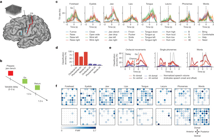
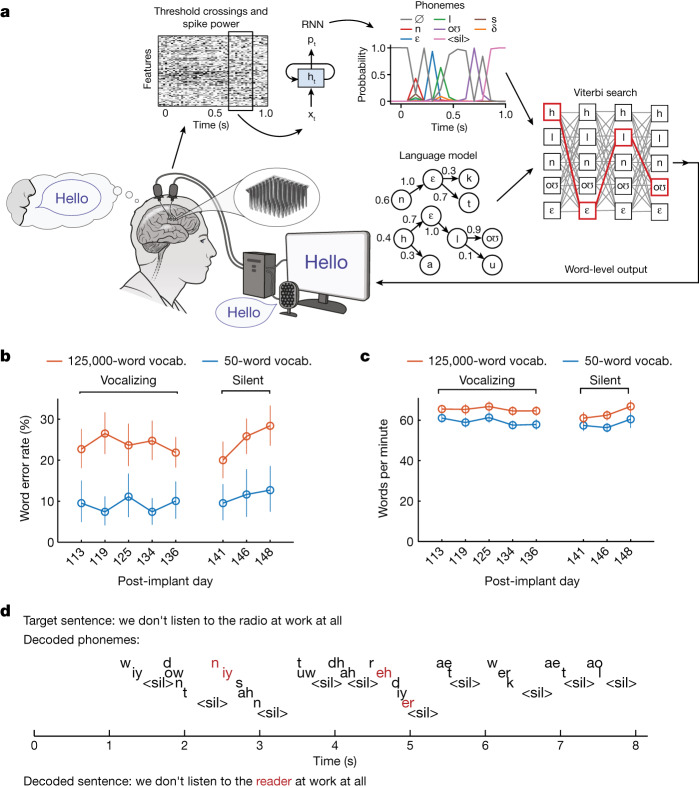
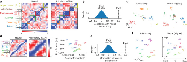
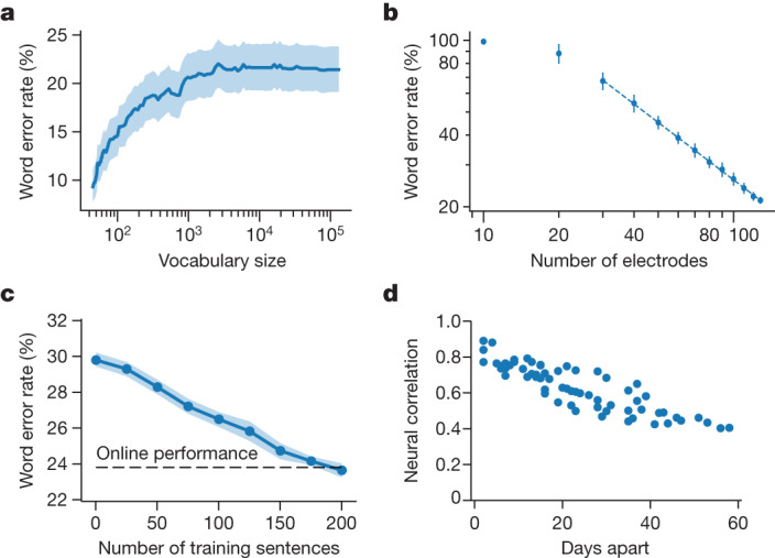
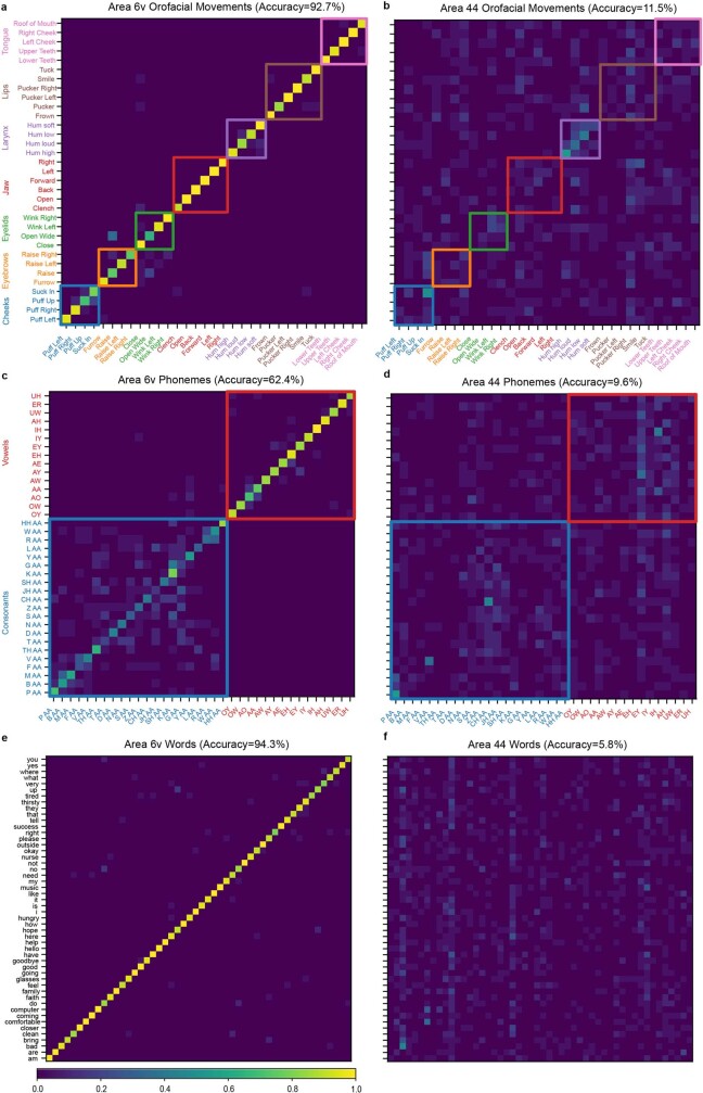
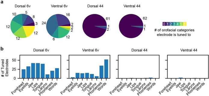
Speech brain-computer interfaces (BCIs) have the potential to restore rapid communication to people with paralysis by decoding neural activity evoked by attempted speech into text^1,2 or sound^3,4. Early demonstrations, although promising, have not yet achieved accuracies sufficiently high for communication of unconstrained sentences from a large vocabulary^1-7. Here we demonstrate a speech-to-text BCI that records spiking activity from intracortical microelectrode arrays. Enabled by these high-resolution recordings, our study participant-who can no longer speak intelligibly owing to amyotrophic lateral sclerosis-achieved a 9.1% word error rate on a 50-word vocabulary (2.7 times fewer errors than the previous state-of-the-art speech BCI²) and a 23.8% word error rate on a 125,000-word vocabulary (the first successful demonstration, to our knowledge, of large-vocabulary decoding). Our participant's attempted speech was decoded at 62 words per minute, which is 3.4 times as fast as the previous record⁸ and begins to approach the speed of natural conversation (160 words per minute⁹). Finally, we highlight two aspects of the neural code for speech that are encouraging for speech BCIs: spatially intermixed tuning to speech articulators that makes accurate decoding possible from only a small region of cortex, and a detailed articulatory representation of phonemes that persists years after paralysis. These results show a feasible path forward for restoring rapid communication to people with paralysis who can no longer speak.

Fig. 1. Neural representation of orofacial movement and attempted speech.

a, Microelectrode array locations (cyan squares) are shown on top of MRI-derived brain anatomy (CS, central sulcus). b, Neural tuning to orofacial movements, phonemes and words was evaluated in an instructed delay task. c, Example responses of an electrode in area 6v that was tuned to a variety of speech articulator motions, phonemes and words. Each line shows the mean threshold crossing (TX) rate across all trials of a single condition (n = 20 trials for orofacial movements and words, n = 16 for phonemes). Shaded regions show 95% confidence intervals (CIs). Neural activity was denoised by convolving with a Gaussian smoothing kernel (80 ms s.d.). d, Bar heights denote the classification accuracy of a naive Bayes decoder applied to 1 s of neural population activity from area 6v (red bars) or area 44 (purple bars) across all movement conditions (33 orofacial movements, 39 phonemes, 50 words). Black lines denote 95% CIs. e, Red and blue lines represent classification accuracy across time for each of the four arrays and three types of movement. Classification was performed with a 100 ms window of neural population activity for each time point. Shaded regions show 95% CIs. Grey lines denote normalized speech volume for phonemes and words (indicating speech onset and offset). f, Tuning heatmaps for both arrays in area 6v, for each movement category. Circles are drawn if binned firing rates on that electrode were significantly different across the given set of conditions (P < 1 × 10^–5 assessed with one-way analysis of variance; bin width, 800 ms). Shading indicates the fraction of variance accounted for (FVAF) by across-condition differences in mean firing rate.

Fig. 2. Neural decoding of attempted speech in real time.

a, Diagram of the decoding algorithm. First, neural activity (multiunit threshold crossings and spike band power) is temporally binned and smoothed on each electrode. Second, an RNN converts a time series of this neural activity into a time series of probabilities for each phoneme (plus the probability of an interword ‘silence’ token and a ‘blank’ token associated with the connectionist temporal classification training procedure). The RNN is a five-layer, gated recurrent-unit architecture trained using TensorFlow 2. Finally, phoneme probabilities are combined with a large-vocabulary language model (a custom, 125,000-word trigram model implemented in Kaldi) to decode the most probable sentence. Phonemes in this diagram are denoted using the International Phonetic Alphabet. b, Open circles denote word error rates for two speaking modes (vocalized versus silent) and vocabulary size (50 versus 125,000 words). Word error rates were aggregated across 80 trials per day for the 125,000-word vocabulary and 50 trials per day for the 50-word vocabulary. Vertical lines indicate 95% CIs. c, Same as in b, but for speaking rate (words per minute). d, A closed-loop example trial demonstrating the ability of the RNN to decode sensible sequences of phonemes (represented in ARPABET notation) without a language model. Phonemes are offset vertically for readability, and ‘<sil>’ indicates the silence token (which the RNN was trained to produce at the end of all words). The phoneme sequence was generated by taking the maximum-probability phonemes at each time step. Note that phoneme decoding errors are often corrected by the language model, which still infers the correct word. Incorrectly decoded phonemes and words are denoted in red.

Fig. 3. Preserved articulatory representation of phonemes.

a, Representational similarity across consonants for neural data (left) and articulatory data from an example subject who can speak normally, obtained from the USC-TIMIT database (right). Each square in the matrix represents pairwise similarity for two consonants (as measured by cosine angle between neural or articulatory vectors). Ordering consonants by place of articulation shows a block-diagonal structure in neural data that is also reflected in articulatory data. b, Neural activity is significantly more correlated with an articulatory representation than would be expected by chance. The blue distribution shows correlations expected by chance (estimated from 10,000 reshufflings of phoneme labels). c, Low-dimensional representation of phonemes articulatorily (left) and neurally (right). Neural data were rotated within the top eight principal components (PC), using cross-validated Procrustes, to show visual alignment with articulatory data. d, Representational similarity for vowels, ordered by articulatory similarity. Diagonal banding in the neural similarity matrix indicates a similar neural representation. For reference, the first and second formants of each vowel are plotted below the similarity matrices. e, Neural activity correlates with the known two-dimensional structure of vowels. f, Same as c but for vowels, with an additional within-plane rotation applied to align the (high versus low) and (front versus back) axes along the vertical and horizontal.

Fig. 4. Design considerations for speech BCIs.

a, Word error rate as a function of language model vocabulary size, obtained by reprocessing the 50-word-set RNN outputs with language models of increasingly large vocabulary size. Word error rates were aggregated over the 250 available trials (50 for each of the five evaluation days). The shaded region indicates 95% CI (computed by bootstrap resampling across trials, n = 10,000 resamplings). b, Word error rate as a function of the number of electrodes included in an offline decoding analysis (each filled circle represents the average word error rate of RNNs trained with that number of electrodes, and each thin line shows s.d. across ten RNNs). There appears to be a log-linear relationship between the number of electrodes and performance, such that doubling the electrode count cuts word error rate by nearly half (factor of 0.57; dashed line represents the log-linear relationship fit with least squares). c, Evaluation data from the five vocalized speech-evaluation days were reprocessed offline using RNNs trained in the same way, but with fewer (or no) training sentences taken from the day on which performance was evaluated. Word error rates averaged across ten RNN seeds (blue line) are reasonable even when no training sentences are used from evaluation day (that is, when training on previous days’ data only). The shaded region shows 95% CI across the ten RNN seeds (bootstrap resampling method, n = 10,000 resamplings). The dashed line represents online performance for reference (23.8% word error rate). d, The correlation (Pearson r) in neural activity patterns representing a diagnostic set of words is plotted for each pair of days, showing high correlations for nearby days.

Extended Data Fig. 1. Example spiking activity recorded from each microelectrode array.

Example spike waveforms detected during a 10-s time window are plotted for each electrode (data were recorded on post-implant day 119). Each 8x8 grid corresponds to a single 64-electrode array, and each rectangular panel in the grid corresponds to a single electrode. Blue traces show example spike waveforms (2.1-ms duration). Neural activity was band-pass filtered (250–5000 Hz) with an acausal, 4^th order Butterworth filter. Spiking events were detected using a −4.5 root mean square (RMS) threshold, thereby excluding almost all background activity. Electrodes with a mean threshold crossing rate of at least 2 Hz were considered to have ‘spiking activity’ and are outlined in red (note that this is a conservative estimate that is meant to include only spiking activity that could be from single neurons, as opposed to multiunit ‘hash’). The results show that many electrodes record large spiking waveforms that are well above the noise floor (the y axis of each panel spans 580 μV, whereas the background activity has an average RMS value of only 30.8 μV). In area 6v,118 electrodes out of 128 had a threshold crossing rate of at least 2 Hz on this particular day (113 electrodes out of 128 in area 44).

Extended Data Fig. 2. Array implant locations and fMRI data shown relative to HCP-identified brain areas.

(a) Array implants shown directly on the brain surface during surgery. (b) Array locations shown on a 3D reconstruction of the brain (array centers shown in blue, yellow, magenta, and orange circles) in StealthStation (Medtronic, Inc.). (c) approximate array locations on the participant’s inflated brain using Connectome Workbench software, overlaid on the cortical areal boundaries (double black lines) estimated by the Human Connectome Project (HCP) cortical parcellation. (d) approximate array locations overlaid on the confidence maps of the areal regions. (e) A language-related resting state network identified in the Human Connectome Project data (N = 210) and aligned to T12’s brain (f) the same resting state network shown in T12’s individual scan. The ventral part of 6v appears to be involved in this resting state network, while the dorsal part is not. This resting state network includes language-related area 55b, Broca’s area and Wernicke’s area.

Extended Data Fig. 3. Classification confusion matrices for orofacial movements, individual phonemes, and individual words.

(a,b) Confusion matrices from a cross-validated, Gaussian naïve Bayes classifier trained to classify amongst orofacial movements using threshold crossing rates averaged in a window from 0 to 1000 ms after the go cue. Each entry (i, j) in the matrix is colored according to the percentage of trials where movement j was decoded (of all trials where movement i was cued). (c,d) Same as a,b but for individual phonemes. (e,f) Same as a,b but for individual words. Matrices on the left show results from using only electrodes in area 6v, while matrices on the right show results from using electrodes in area 44. Although good classification performance can be observed from area 6v, area 44 appears to contain little to no information about most movements, phonemes and words.

Extended Data Fig. 4. Individual microelectrodes are tuned to multiple categories of orofacial movement.

(a) Pie charts summarizing the number of electrodes that had statistically significant tuning to each possible number of movement categories (from 0 to 6), as assessed with a 1-way ANOVA (p < 1e-5). On the 6v arrays, many electrodes are tuned to more than one orofacial movement category (forehead, eyelids, jaw, lips, tongue, and larynx). (b) Bar plots summarizing the number of tuned electrodes to each movement category and each array. The ventral 6v array contains more electrodes tuned to phonemes and words, while the dorsal 6v array contains more electrodes tuned to orofacial movement categories. Nevertheless, both 6v arrays contain electrodes tuned to all categories of movement.

Extended Data Fig. 5. Offline parameter sweeps show the effect of RNN parameters and architecture choices.

Black arrows denote the parameters used for real-time evaluation. Blue open circles show the performance of single RNN seeds, while thin blue bars denote the mean across all seeds. (a) Rolling z-scoring improves performance substantially relative to no feature adaptation (when testing on held-out blocks that are separated in time from the training data). (b) Training RNNs with day-specific input layers improves performance relative to using a shared layer across all days. (c) RNN performance using different neural features as input (SP=spike band power, TX=threshold crossing). Combining spike band power with threshold crossings performs better than either alone. It appears that performance could have been improved slightly by using a −3.5 RMS threshold instead of −4.5. (d) RNN performance using audio-derived mel frequency cepstral coefficients (“audio MFCC”) or neural features from the area 44 arrays. While the MFCCs yield poor but above-chance performance, word error rates from IFG recordings appear to be at chance level (~100%). (e) RNN performance as a function of “kernel size” (i.e., the number of 20 ms bins stacked together as input and fed into the RNN at each time step). It appears that performance could have been improved by using larger kernel sizes. (f) RNN performance as a function of “stride” (a stride of N means the RNN steps forward only every N time bins). (g) RNN performance as a function of the number of stacked RNN layers. (h) RNN performance as a function of the number of RNN units per layer. (i) RNN performance as a function of the number of prior days included as training data. Performance improves by adding prior days, but with diminishing returns. The blue line shows the average word error rate across 10 RNN seeds and 5 evaluation days. Vertical lines show standard deviations across the 10 seeds.

Extended Data Fig. 6. Phoneme substitution errors observed across all real-time evaluation sentences.

Entry (i.j) in the matrix represents the substitution count observed for true phoneme i and decoded phoneme j. Substitutions were identified using an edit distance algorithm that determines the minimum number of insertions, deletions, and substitutions required to make the decoded phoneme sequence match the true phoneme sequence. Most substitutions appear to occur between phonemes that are articulated similarly.

Extended Data Fig. 7. Contribution of each array and microelectrode to decoding performance.

(a) Word error rates for a retrospective offline decoding analysis using just the ventral 6v array (left column), dorsal 6v array (middle column), or both arrays (right column). Each circle indicates the word error rate for one of 10 RNN seeds. Word error rates were aggregated across 400 trials. Horizontal lines depict the mean across all 10 seeds. (b) Heatmaps depicting the (offline) increase in phoneme error rate when removing each electrode from the decoder by setting the values of its corresponding features to zero. Results were averaged across 10 RNN seeds that were originally trained to use every electrode. Almost all electrodes seem to contribute to decoding performance, although the most informative electrodes are concentrated on the ventral array. The effect of removing any one electrode is small (<1% increase in phoneme error rate), owing to the redundancy across electrodes.

Extended Data Fig. 8. Additional methods and able-bodied subjects provide further evidence for an articulatory neural code.

(a) Representational similarity across consonants (top) and vowels (bottom) for different quantifications of the neural activity (“Saliency Vectors”, “Decoder Labels”, and “Single Phoneme Task”) and articulator kinematics (“Haskins M01”, “USC-Timit M1”, “Place + Formants”). Each square in a matrix represents pairwise similarity for two phonemes (as measured by the cosine angle between the neural or articulatory vectors). Consonants are ordered by place of articulation (but with approximants grouped separately) and vowels are ordered by articulatory similarity (as measured by “USC-TIMIT M1”). These orderings reveal block-diagonal structure in the neural data that is also reflected in articulatory data. “Haskins M01” and “USC-Timit M1” refer to subjects M01 and M1 in the Haskins and USC-Timit datasets. “Place + Formants” refers to coding consonants by place of articulation and to representing vowels using their two formant frequencies. (b) Correlations between the neural representations and the articulator representations (each panel corresponds to one method of computing the neural representation, while each column corresponds to one EMA subject or the place/formants method). Orange dots show the correlation value (Pearson r), and blue distributions show the null distribution computed with a shuffle control (10,000 repetitions). In all cases, the true correlation lies outside the null distribution, indicating statistical significance. Correlation values were computed between consonants and vowels separately and then averaged together to produce a single value. (c) Representational similarity matrices computed using the “Decoder labels” method on 6 different independent folds of the neural data. Very similar representations across folds indicates that the representations are statistically robust (average correlation across folds = 0.79).

References

1. Herff C, et al. Brain-to-text: decoding spoken phrases from phone representations in the brain. Front. Neurosci. 2015;9:217. doi: 10.3389/fnins.2015.00217. - DOI - PMC - PubMed
1. Moses DA, et al. Neuroprosthesis for decoding speech in a paralyzed person with anarthria. N. Engl. J. Med. 2021;385:217–227. doi: 10.1056/NEJMoa2027540. - DOI - PMC - PubMed
1. Anumanchipalli GK, Chartier J, Chang EF. Speech synthesis from neural decoding of spoken sentences. Nature. 2019;568:493–498. doi: 10.1038/s41586-019-1119-1. - DOI - PMC - PubMed
1. Herff C, et al. Generating natural, intelligible speech from brain activity in motor, premotor, and inferior frontal cortices. Front. Neurosci. 2019;13:1267. doi: 10.3389/fnins.2019.01267. - DOI - PMC - PubMed
1. Kellis S, et al. Decoding spoken words using local field potentials recorded from the cortical surface. J. Neural Eng. 2010;7:056007. doi: 10.1088/1741-2560/7/5/056007. - DOI - PMC - PubMed
Publication types