Excitatory/inhibitory balance emerges as a key factor for RBN performance, overriding attractor dynamics

Abstract

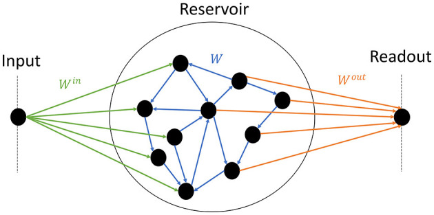
Reservoir computing provides a time and cost-efficient alternative to traditional learning methods. Critical regimes, known as the "edge of chaos," have been found to optimize computational performance in binary neural networks. However, little attention has been devoted to studying reservoir-to-reservoir variability when investigating the link between connectivity, dynamics, and performance. As physical reservoir computers become more prevalent, developing a systematic approach to network design is crucial. In this article, we examine Random Boolean Networks (RBNs) and demonstrate that specific distribution parameters can lead to diverse dynamics near critical points. We identify distinct dynamical attractors and quantify their statistics, revealing that most reservoirs possess a dominant attractor. We then evaluate performance in two challenging tasks, memorization and prediction, and find that a positive excitatory balance produces a critical point with higher memory performance. In comparison, a negative inhibitory balance delivers another critical point with better prediction performance. Interestingly, we show that the intrinsic attractor dynamics have little influence on performance in either case.

Keywords: RBN; attractor; criticality; memory; prediction; reservoir computing.

Figure 1

Schematics of the model. The input node (left) randomly projects synaptic weights to half of the reservoir (center) (green); the reservoir is composed of random recurrent connections (blue); the readout (right) receives input from the other half of the reservoir (orange).

Figure 2

Excitation/inhibition balance b as a function of the absolute value of the connectivity parameter σ^⋆, as defined in Eq. 4, for σ^⋆ < 0 $\left(\mathrm{—}\right)$ and σ^⋆> 0 $\left(\mathrm{—}\right)$. When the average of weights is positive (σ^⋆> 0), whereas the reverse is true when the average of weights is negative.

Figure 3

Statistics of the activity of free running reservoirs in the steady state as a function of |σ^⋆|. Each dot represents the statistics over 100 reservoirs ran once. Average over reservoirs of time average activity 〈Ā〉 (A), and average over reservoir of time variance $\langle \overline{\delta A^2}\rangle$ (C), for σ^⋆ < 0 ($\mathrm{▾}$) and σ^⋆> 0 ($\mathrm{▴}$). In all plots, the gray vertical lines represent the critical values of the control parameter for ${\sigma }_c^{\star }<0$ (---) and ${\sigma }_c^{\star }>0$ (-.-.). (B, D) Zoom on the region of interest close to the critical points: average over reservoirs of BiEntropy 〈H_b〉 (⋆, left scale) and BiEntropy variance $\langle \delta H_b^2\rangle$ ($\mathrm{•}$, right scale), for σ^⋆ < 0 (B) and σ^⋆> 0 (D).

Figure 4

The attractor landscape of reservoirs: for σ^⋆ < 0 (A–C, G), and for σ^⋆> 0 (D–F, H). The influence of initial conditions for specific values of σ^⋆: (A) σ^⋆ = −0.6, (B) σ^⋆ = −0.66, (C) σ^⋆ = −0.689, (D) σ^⋆ = 2.4, (E) σ^⋆ = 4.0, (F) σ^⋆ = 5.0. In each plot, the vertical axis represents different numbers (#) of initial random states of free-running reservoirs. The horizontal axis represents different numbers (#) of reservoirs with various initial weight tossing, randomly generated with distinct seeds. Pixels of colors represent the attractor obtained at the steady state, with the same colors as (G, H). (G, H) Percentage of steady-state activities belonging to each category of attractors: no-activity ($\mathrm{+}$), fix ($\mathrm{•}$), cyclic ($\mathrm{•}$), and irregular ($\mathrm{♦}$). Each dot represents the statistics over 100 reservoirs ran 100 times, hence 1, 000 runs. In each row (A–C, E–G), the colored dashed boxes surrounding the plots correspond to the values of σ^⋆, indicated as vertical lines in plots (G, H).

Figure 5

Performances for two tasks: white noise memory (C, E); and Mackey-glass prediction (D, F). (A, D) Examples of signals for each task with their respective parameters. (A) White noise memory task, which consists in remembering the input (gray), to reproduce it in output (dark red) with a negative delay δ (shown example corresponds to δ = −6). (B) Mackey glass is controlled by the parameter τ (see methodology Supplementary material S8.3 for more details), ranging from periodic to chaotic. (C–F) The average performance Corr(y, T) between the output y and target T, plotted over |σ^⋆|, for each dominant attractor category no-activity, fix, cyclic or irregular. For each value of σ^⋆ we have 100 reservoirs. The solid line then represents the average over reservoirs belonging to the same attractor category; individual reservoir performances are averaged over 5 initial conditions. The shaded area represents one standard deviation. Higher correlations indicate better performance. The hatched gray area represents the critical regions, as defined in Section 3.1. (C, D) The performance in the white-noise memory task; three values of δ are tested −2 (⋆), −6 (•), −10 (▾). (E, F) The performance of Mackey-Glass prediction (δ = +10); three values of τ are tested 5 (⋆), 20 (⋆), and 50 (▾). (C, D) Performance for σ^⋆ < 0, with inside each plot a zoom on the critical region. (E, F) Performance for σ^⋆> 0.

Figure 6

The performance of all reservoirs in the prediction tasks (Mackey-Glass) as a function of their performance in the memory tasks (white-noise), for σ^⋆ < 0 (A–C) and σ^⋆> 0 (D–F). Reservoirs are again classified according to their dominant attractor (see Supplementary material S13). Each dot represents an individual reservoir performance averaged over 5 initial conditions. In all plots, dots with black edges display reservoirs taken at the critical regimes. We chose three different pairs of values for the parameters of the tasks, τ and δ, each representing a different difficulty level: 1. Simple (A, D) the lowest difficulty in both tasks, τ = 5 and δ = −2; 2. Average (B, E) average difficulty for intermediary values of τ = 20 and δ = −6; 3. Difficult (C, F) difficult task for higher values of τ = 28 and δ = −10.

References

1. Alexandre L. A., Embrechts M. J., Linton J. (2009). “Benchmarking reservoir computing on time-independent classification tasks,” in Proceedings of the International Joint Conference on Neural Networks 89–93. 10.1109/IJCNN.2009.5178920 - DOI
1. Balafrej I., Alibart F., Rouat J. (2022). P-CRITICAL: a reservoir autoregulation plasticity rule for neuromorphic hardware. Neuromor. Comput. Eng. 2, 024007. 10.1088/2634-4386/ac6533 - DOI
1. Benjamin B. V., Gao P., McQuinn E., Choudhary S., Chandrasekaran A. R., Bussat J.-M., et al. . (2014). Neurogrid: a mixed-analog-digital multichip system for large-scale neural simulations. Proc. IEEE 102, 699–716. 10.1109/JPROC.2014.2313565 - DOI
1. Bertschinger N., Natschläger T. (2004). Real-time computation at the edge of chaos in recurrent neural networks. Neur. Comput. 16, 1413–1436. 10.1162/089976604323057443 - DOI - PubMed
1. Bianchi F. M., Livi L., Alippi C. (2016). Investigating echo state networks dynamics by means of recurrence analysis. IEEE Trans. Neur. Netw. Learn. Syst. 29, 427–439. 10.1109/TNNLS.2016.2630802 - DOI - PubMed