Modular architecture facilitates noise-driven control of synchrony in neuronal networks

Abstract

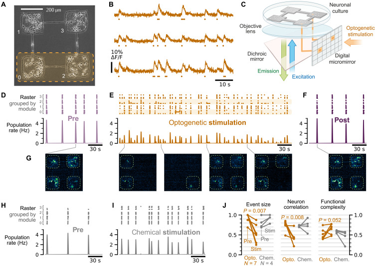
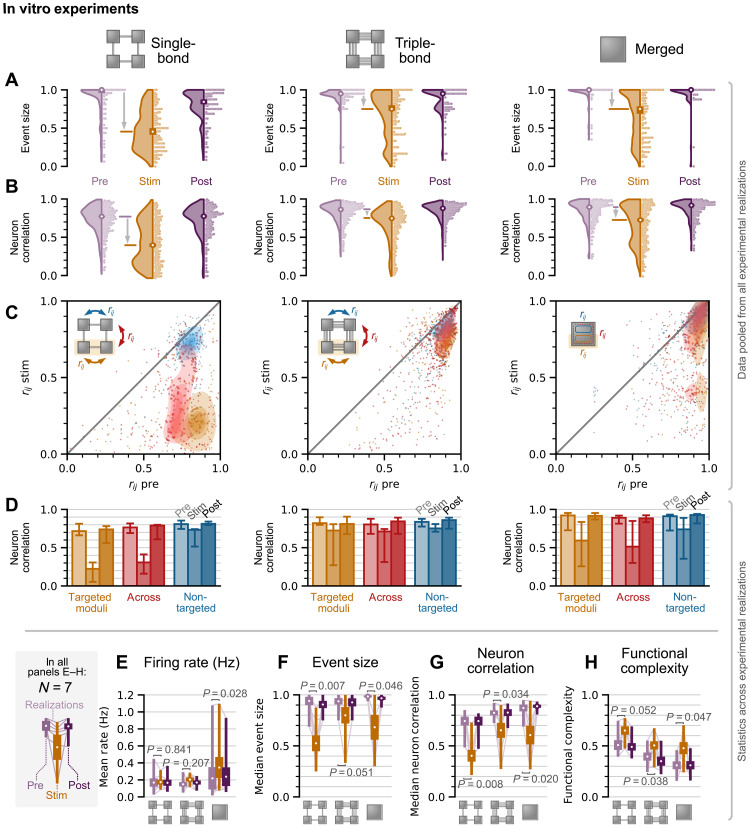
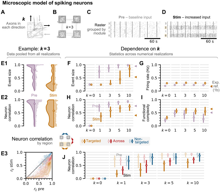
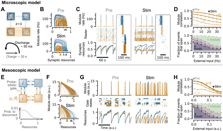
High-level information processing in the mammalian cortex requires both segregated processing in specialized circuits and integration across multiple circuits. One possible way to implement these seemingly opposing demands is by flexibly switching between states with different levels of synchrony. However, the mechanisms behind the control of complex synchronization patterns in neuronal networks remain elusive. Here, we use precision neuroengineering to manipulate and stimulate networks of cortical neurons in vitro, in combination with an in silico model of spiking neurons and a mesoscopic model of stochastically coupled modules to show that (i) a modular architecture enhances the sensitivity of the network to noise delivered as external asynchronous stimulation and that (ii) the persistent depletion of synaptic resources in stimulated neurons is the underlying mechanism for this effect. Together, our results demonstrate that the inherent dynamical state in structured networks of excitable units is determined by both its modular architecture and the properties of the external inputs.

Fig. 1.. Optogenetic stimulation on modular neuronal cultures increases the variability in collective network dynamics.

(A) Phase-contrast image of a representative single-bond modular network. Neurons appear as dark round objects with a white contour. Ten neurons were selected from the bottom module pair (orange box) and optogenetically targeted in a random manner. (B) Representative fluorescence traces and inferred spike events (dots) of three neurons along 1 min. (C) Sketch of the experimental setup. Neuronal cultures were transfected with ChrimsonR for optogenetic stimulation (orange arrow) and GCaMP6s for simultaneous activity monitoring (blue and green arrows). (D) Pre-stimulation raster plot (top panel) of network spontaneous activity, with neurons grouped according to their module, and the corresponding population activity (bottom). (E) Corresponding data upon optogenetic stimulation, wherein population activity markedly increases in variability. Targeted modules are marked as orange bands. (F) Spontaneous activity post-stimulation, with a return to strong network-wide bursting. (G) Representative snapshots of calcium imaging recordings for the above data. All modules activate synchronously without stimulation. Upon stimulation, activity events extend over individual neurons, multiple modules, or all modules. (H and I) Raster plot and population activity before and during chemical stimulation. Chemical stimulation increases the frequency of events but maintains the network-wide activity. (J) Effect of optogenetic and chemical stimulation on bursting median event sizes, median correlation coefficients, and functional complexity (paired-sample t test, two-sided). For chemical stimulation with N = 4, no test was performed.

Fig. 2.. Disruption of network-wide collective activity upon optogenetic stimulation is facilitated by modular architecture.

(A) From left to right, event size distribution before, during, and after optogenetic stimulation for the 1-b, 3-b, and merged networks. Violin plots (left side of distribution) represent smooth kernel estimates of the events observed across all networks, while individual observations are shown in swarms (right side). Error bars (middle) are obtained via bootstrapping. White dots indicate the median of the 500 bootstrap estimates, and bars represent the 95 percentiles. (B) Corresponding distribution of pairwise Pearson correlation coefficients between neurons calculated from binned spike counts. A substantial drop is only observed for 1-b. Data are presented as in (A). (C) Change of correlation coefficients r_ij between the pre-stimulated and stimulated conditions, grouped according to the regions in which neurons are located. Both neurons may either reside in regions that are targeted by stimulation (yellow), both reside in nontargeted regions (blue), or the pair spans across a targeted and nontargeted regions (red). For modular networks, the regions correspond directly to modules. Decorrelation is more pronounced when one or both neurons are in regions that are targeted. Colored areas are fitted probability density estimates for each data group. (D) Same as (C) but showing realization-level statistics. Bar heights represent the medians of independent estimates in each realization, and error bars represent 95 percentiles. cf. table S7. (E to H) Estimates for each realization: mean firing rates (E), median event sizes (F), median correlation coefficients (G), and functional complexity (H) for the three topologies. Thin lines, individual realizations (networks); white dots, means of 500 bootstrap samples; thick bars, SEM; thin bars, extrema. P values are from paired-sample t test (two-sided), cf. tables S1 and S7.

Fig. 3.. Microscopic-level simulations of modular networks using LIF neuron models.

(A) Sketch of a single module, where k axons connect to each adjacent neighbor (shown for k = 1). (B) Sketch of a simulated modular network with k = 3. (C and D) Representative raster plots in the pre-stimulated (C) and stimulated (D) regimes. Modules targeted with an increased noise are #0 and #2. (E1 and E2) Joint distributions of event size and pairwise correlation coefficients from data pooled from 50 independent numerical realizations, comparing pre and stim conditions. Both distributions exhibit a substantial drop towards smaller values upon stimulation. White dots are the median of 500 bootstrap estimates, and error bars representing the 95 percentiles are smaller than the symbol size. (E3) Change of correlation coefficients r_ij between the pre-stimulated and stimulated conditions (yellow: neuronal pairs reside in target modules; blue: reside in nontargeted; red: span across a target and a nontargeted module). The diagonal black line is the no-change reference condition. As in the experiments, decorrelation is more pronounced when one or both neurons are in modules with increased noise. (F to I) Dependence of four descriptors (event size, firing rate, neuron correlation, and functional complexity) on k. The higher k, the lower the modularity of the networks. Statistics are obtained across realizations where each realization yields a single scalar. White dots are the median of single-realization estimates. Rounded bars are 68 percentiles, indicating the variability between realizations. Triangles on the right of each panel indicate the values from single-bond experiments. (J) Correlation of neuron pairs grouped by the neurons’ respective modules (yellow, red, and blue). For each k, the pre- and post-conditions are compared (faint versus dark colors). The strongest decorrelation is observed when both neurons are in noise-targeted modules (yellow) or modularity is high (k = 1 and 3).

Fig. 4.. Desynchronization can be understood through charge-discharge cycles in the resource-rate plane, which is captured by a minimal mesoscopic model.

(Top row) Microscopic model using LIF neurons. (Bottom row) Mesoscopic model, where modules are the smallest functional unit. (A) Top: Sketch of the microscopic model, in which orange modules are those targeted by an increased noise. Bottom: Conceptual representation of the resource-rate cycles and the contrasting timescales involved. (B) Resource-rate cycles in a representative simulation with k = 3. Orange trajectories correspond to targeted modules, and blue trajectories correspond to nontargeted ones. Under stimulation, resources are more depleted on average (smaller excursions), and discharge events start at lower resources (colored triangles). (C) Module-level firing rates, raster plot, and average module-level resources under pre and stim conditions. Insets show a detail of neuronal activity during a network-wide activity event. (D) Top: Correlation between module-level firing rates of targeted modules as a function of the external input (added noise). Curves from bottom to top correspond to gradually higher k values. Triangles indicate the the values of external input for the pre and stim conditions, from which the cycles and raster plots of (B) and (C) are built. Bottom: Average fraction of modules that participate in an event for k = 3 as a function of external input. (E) Top: Sketch of the mesoscopic model with probabilistic gates between modules. Bottom: Gates have a high probability to disconnect when resources of the source module are low. (F) Resource-rate cycles and the effect of stimulation for the mesoscopic model. (G) Module rate, gate state (solid when connected), and module resources as a function of time. Note the disconnection of gates after high-rate discharge events. (H) Top: Correlation of the firing rates of targeted modules as a function of the external input. Bottom: Average fraction of modules involved in events (w = 0.1). a.u., arbitrary units.

References

1. W. R. Softky, C. Koch, The highly irregular firing of cortical cells is inconsistent with temporal integration of random EPSPs. J. Neurosci. 13, 334–350 (1993). - PMC - PubMed
1. A. Arieli, A. Sterkin, A. Grinvald, A. D. Aertsen, Dynamics of ongoing activity: Explanation of the large variability in evoked cortical responses. Science 273, 1868–1871 (1996). - PubMed
1. M. E. Raichle, The restless brain. Brain Connect. 1, 3–12 (2011). - PMC - PubMed
1. J. Aru, J. Aru, V. Priesemann, M. Wibral, L. Lana, G. Pipa, W. Singer, R. Vicente, Untangling cross-frequency coupling in neuroscience. Curr. Opin. Neurobiol. 31, 51–61 (2015). - PubMed
1. A. Fornito, A. Zalesky, E. Bullmore, in Fundamentals of brain network analysis. (Academic Press, 2016).