Geometric framework to predict structure from function in neural networks

Abstract

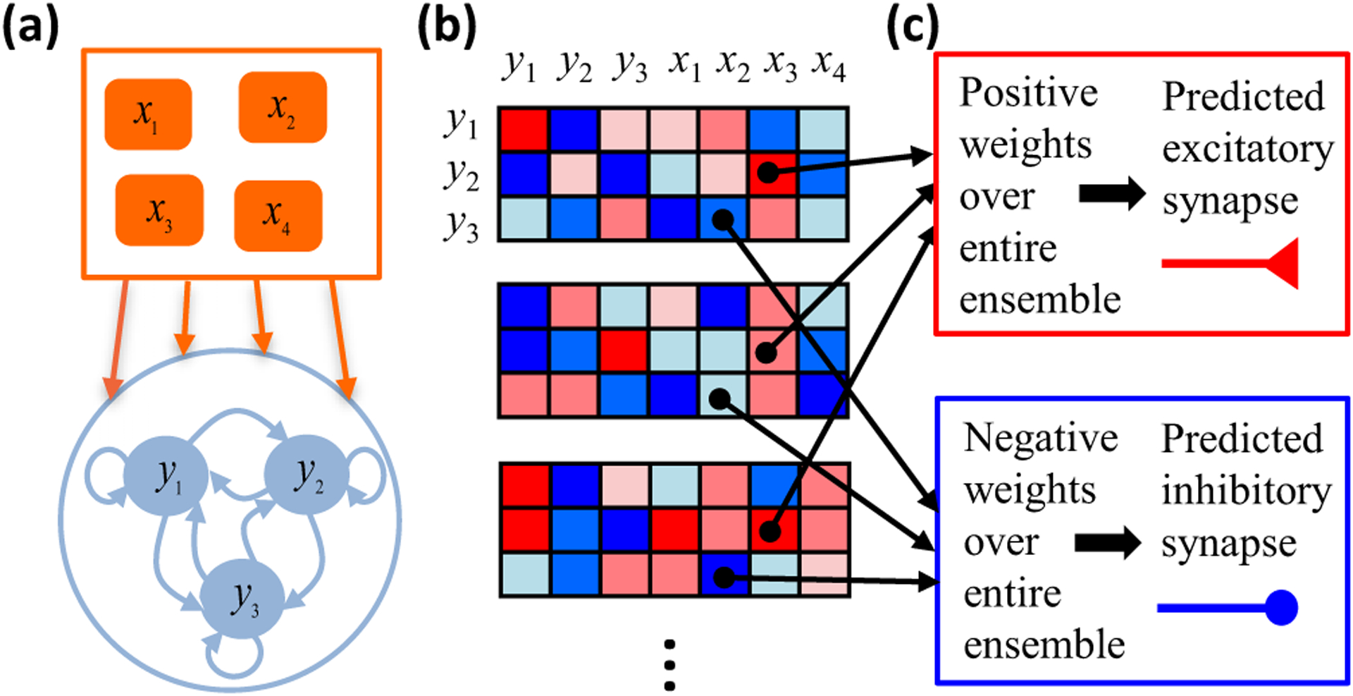
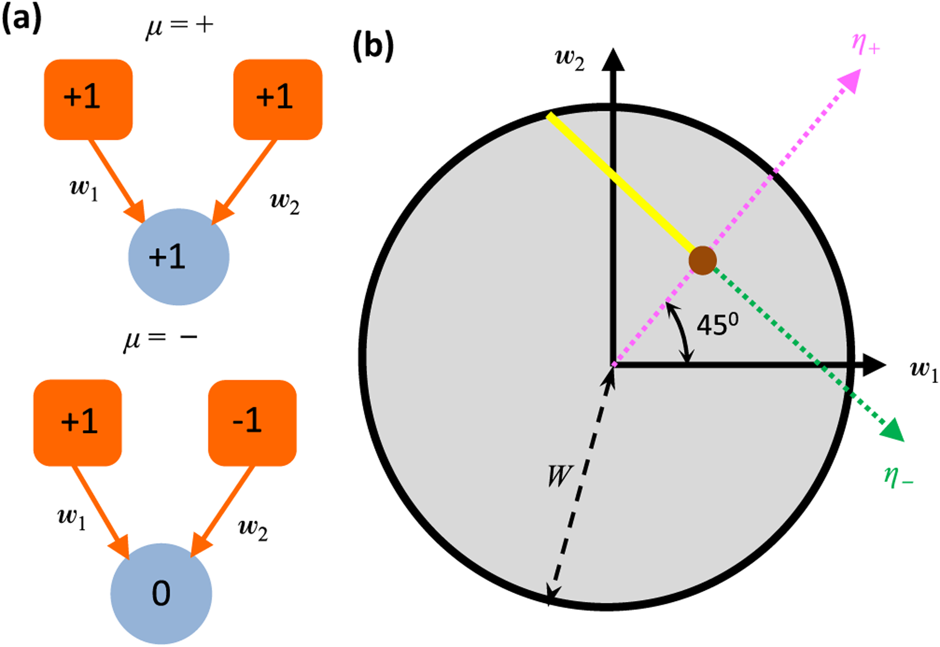
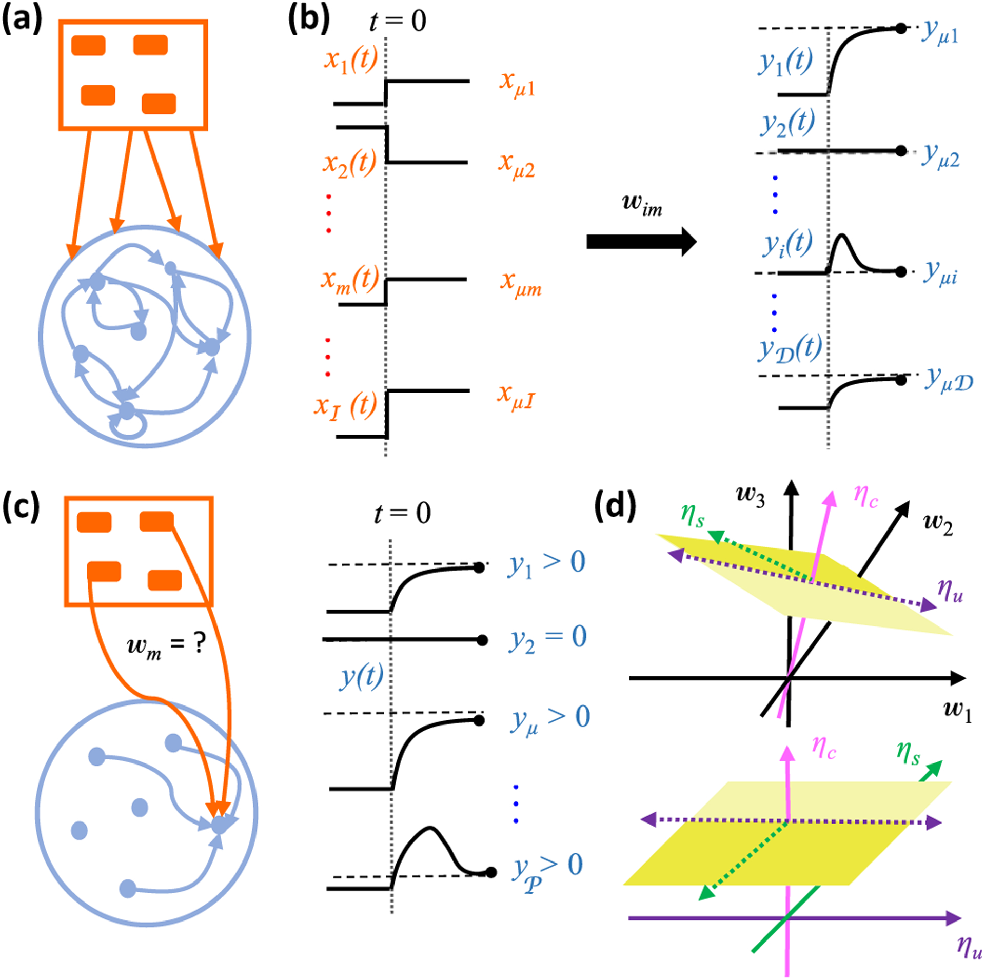
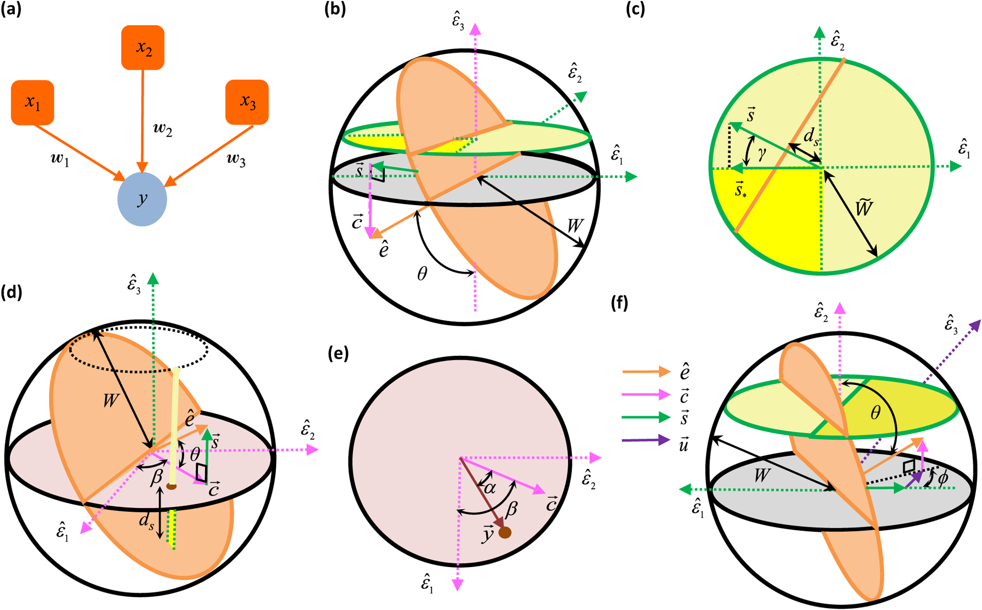
Neural computation in biological and artificial networks relies on the nonlinear summation of many inputs. The structural connectivity matrix of synaptic weights between neurons is a critical determinant of overall network function, but quantitative links between neural network structure and function are complex and subtle. For example, many networks can give rise to similar functional responses, and the same network can function differently depending on context. Whether certain patterns of synaptic connectivity are required to generate specific network-level computations is largely unknown. Here we introduce a geometric framework for identifying synaptic connections required by steady-state responses in recurrent networks of threshold-linear neurons. Assuming that the number of specified response patterns does not exceed the number of input synapses, we analytically calculate the solution space of all feedforward and recurrent connectivity matrices that can generate the specified responses from the network inputs. A generalization accounting for noise further reveals that the solution space geometry can undergo topological transitions as the allowed error increases, which could provide insight into both neuroscience and machine learning. We ultimately use this geometric characterization to derive certainty conditions guaranteeing a nonzero synapse between neurons. Our theoretical framework could thus be applied to neural activity data to make rigorous anatomical predictions that follow generally from the model architecture.

FIG. 1.

Cartoon of theoretical framework. (a) We first specify some steady-state responses of a recurrent threshold-linear neural network receiving feedforward input. (b) We then find all synaptic weight matrices that have fixed points at the specified responses. Red (blue) matrix elements are positive (negative) synaptic weights. (c) When a weight is consistently positive (or consistently negative) across all possibilities, then the model needs a nonzero synaptic connection to generate the responses. We therefore make the experimental prediction that this synapse must exist. We also predict whether the synapse is excitatory or inhibitory.

FIG. 2.

An illustrative two-dimensional problem. (a) Cartoon depicting two stimulus response patterns in a simple feedforward network with two input neurons and one driven neuron. (b) Since the driven neuron in panel (a) responds in one condition but not the other, we have one constrained dimension (magenta axis) and one semiconstrained dimension (green axis). The yellow ray depicts the space of weights, (w₁, w₂), that generate the stimulus transformation. The weight vector $\left(\frac{1}{2},\frac{1}{2}\right)$ (brown dot) would uniquely generate the neural responses in a linear network. We assume that the magnitude of the weight vector is bounded by W, such that all candidate weight vectors lie within a circle of that radius. A nonzero synapse x₂ → y exists in all solutions, but the x₁ → y synapse can be zero because the yellow ray intersects the w₁ = 0 axis.

FIG. 3.

Finding network structure that implements functional responses. (a) Cartoon depicting a recurrent network of driven neurons (blue) receiving feedforward input from a population of input neurons (orange). (b) The μth pattern of input neuron activity (x_μm) appears at t = 0 and drives the recurrent neurons to approach the steady-state response pattern (y_μi) via feedforward and recurrent network connectivity (w_im). (c) (Left) We focus on one driven neuron at a time, referred to henceforth as the target neuron, to determine its possible incoming synaptic weights, w_m. (Right) These weights must reproduce the target neuron’s 𝒫 steady-state responses from the steady-state activity patterns of all 𝒩 presynaptic neurons. (d) The yellow planes depict the subspace of incoming weights that can exactly reproduce all nonzero responses of the target neuron, and the subregion shaded dark yellow indicates weights that also reproduce the target neuron’s zero responses. The top graph depicts the weight space parametrized by physically meaningful w coordinates, but the solution space is more simply parametrized by abstract η coordinates (bottom). The η coordinates depend on the specified stimulus transformation (x_μm → y_μi), and η_c, η_s, and η_u are coordinates in 𝒞-dimensional constrained, 𝒮-dimensional semiconstrained, and 𝒰-dimensional unconstrained subspaces, respectively.

FIG. 4.

Geometric quantities determining whether neurons must be synaptically connected in several three-dimensional toy problems. (a) Cartoon depicting the 𝒩 = 3 feedforward network corresponding to the toy problems. (b), (c) Geometrically determining whether a synapse is nonzero when the target neuron responds to one input pattern but does not to two other patterns. A synapse can only vanish if the w₁ = 0 plane (orange circle) intersects the solution space (dark yellow wedge) within the weight bounds (bounding sphere). For example, this intersection occurs in panel (b), so the synapse is not required for the responses. For every synapse one can associate a direction in synaptic weight space (orange arrow) that is normal to the planes with constant synaptic weight. This synapse vector can be decomposed into its projections into the semiconstrained subspace (green arrow, $\overrightarrow{s}$) and along the constrained dimension (pink arrow, $\overrightarrow{c}$). In this example, whether the synapse is certain is determined by the size of the bounding synapse space, W [see panel (b)], the angle θ between the synapse direction (orange arrow) and the closest axis of the constrained dimension $\left(-{\overrightarrow{\epsilon }}_3\right)$ [see panel (b)], and the angle γ between $\overrightarrow{s}$ and its closest vector in the solution space $\left({\overrightarrow{s}}_{\ast }\right)$ [see panel (c)]. In panel (c), d_s depicts the perpendicular distance from the origin of the yellow semiconstrained plane in panel (b) to its intersection line with the w₁ = 0 orange plane. If this distance is sufficiently large, then the orange line will not intersect the target neuron responds to two input patterns but not the third pattern. In panel (d), the orange w₁ = 0 plane intersects the solution space (deep solution space within the yellow plane’s circular bound of radius $\tilde{W}$. (d), (e) Geometrically determining whether a synapse is nonzero when the yellow line) within the bounding sphere, so the synapse is not certain. In this example, the factors that determine synapse certainty are W [see panel (d)], the angle θ that the synapse vector (orange arrow) makes with its projection along the constrained subspace (pink arrow) [see panel (d)], and the angle α between the target response vector (brown arrow) and the pink arrow [see panel (e)]. The angle β does not ultimately matter, but it is included in the diagrams to aid the derivation. Here d_s is the distance from the brown dot to the point of intersection between the yellow line and the orange plane. Again this point will lie outside the bounding sphere if d_s is large enough, and this signals a certain synapse. (f) Geometrically determining whether a synapse is nonzero when the target neuron responds to one input pattern but does not to a second pattern. In the figure shown, the w₁ = 0 orange plane intersects the solution space (deep yellow semicircle) within the bounding sphere, so the synapse is not certain. In this example, apart from W, what determines synapse certainty are the angles θ and φ, which encode how the synapse vector (orange arrow) can be decomposed into its projections along the constrained direction (pink arrow), semiconstrained direction (green arrow) and unconstrained direction (purple arrow).

FIG. 5.

Identifying certain synapses in high-dimensional networks. (a) Cartoon depicting the high-dimensional feedforward network under consideration. (b) Geometrically determining whether a synapse is nonzero throughout a high-dimensional solution space. A synapse can only vanish if the w_m = 0 hyperplane (orange circle) intersects the solution space (dark yellow wedge) within the weight bounds (bounding sphere). In the example shown, this intersection does not occur, so the synapse must be present. For orthonormal neural responses, only a few parameters determine whether this intersection occurs (Appendix A). First, the magnitude of the weight bound, W, controls the extent of the solution space. Second, there are three projections of the synapse direction (orange arrow) whose lengths are important determinants of the certainty condition: e_y, the length of projection along the target response vector (pink arrow); e_s*, the length of projection along the closest boundary vector in the semiconstrained solution subspace [green arrow, see also ${\overrightarrow{s}}_{\ast }$ in Fig. 4(c)]; and e_u, the length of projection into the unconstrained subspace (purple arrow). Note that the shown example would have had an intersection if the solution space (dark yellow wedge) were moved down (along $\widehat{c}$) to lie below the hyperplane (orange circle). The solution space’s height is proportional to the magnitude of the postsynaptic responses, y. Thus, the solution space does not intersect the hyperplane only if y exceeds a critical value, y_cr. (c) Plots of the certainty condition, Eq. (57), for W = 1. The red, blue, and purple curves plot y_cr as a function of r_y = e_y/e_p for e_p = 0.3, 0.6, and 0.9, respectively. Different purple shades correspond to different values of $r_{s\ast }=e_{s\ast }/\sqrt{e_p^2-e_y^2}$. As this ratio increases, nonlinear effects increase y_cr and make the sign harder to determine. The red and blue curves are for the maximally nonlinear case when $r_{s\ast }=1\Rightarrow e_{s\ast }=\sqrt{e_p^2-e_y^2}$. The dashed black curves represent y_cr in a linear model, which cannot exceed the nonlinear y_cr.

FIG. 6.

Testing the certainty condition with exhaustive low-dimensional simulations. (a) A simple recurrent network with three input neurons and three driven neurons (Appendix E). (b) We plot the theoretically derived y_cr for feedforward synapses to y₁ as we vary θ (green curves) or φ (magenta curves), keeping the other angle fixed at 45°. The lighter shades correspond to cosγ = 1 ⇒ r_s* = 1. The darker shades correspond to cosγ = 0 ⇒ r_s* = 0, where the predictions from the nonlinear network match those of a linear network. The dots represent y_cr estimated through simulations, and they agree well with the theory. (c) (Bottom) Bar graph of the fraction of solutions with positive (red) and negative (blue) self-couplings (y₃ → y₃) as a function of θ. (Top) As predicted, all solutions have positive w_y3,y3 when y − y_cr > 0.

FIG. 7.

The solution space geometry changes as the allowed error increases. (a) Error surface contours in a three-dimensional subspace corresponding to η₁, η₂, and η₃. Several topological transitions occur as the error increases. (i) We consider the case where all responses are positive, so the contours are spherical for small errors, just like in a linear neural network. (ii), (iii) Two cylindrical dimensions sequentially open up when the error is large enough for some η coordinates to become negative. (iv), (v) After that, either a third cylindrical dimension can open up, or the two cylindrical axes can join to form a plane. Which transition occurs at lower error depends on the pattern of neural responses. (b) (Left) We illustrate a case where there is a unique exact solution to the problem (brown dot). Allowing error but neglecting topological transitions would expand the solution space to an ellipse (here, brown circle), but the signs of w₁ and w₂ remains positive. Including topological transitions in the error surface can cap the ellipse with a cylinder (full yellow solution space). Now we can say with certainty that the sign of w₂ is positive, but negative values of w₁ become possible. (Right) Graphical conventions are the same. However, in this case all solutions inside the cylinder have w₂ > 0. Therefore, the topological transition breaks a near symmetry between positive and negative weights.

FIG. 8.

The theory accounting for error explains numerical ensembles of feedforward and recurrent networks. (a) Cartoon of a recurrent neural network. We disallow recurrent connectivity of neurons onto themselves throughout this figure. 𝒟 = 1 corresponds to the feedforward case, and W = 1 for all panels. (b) Comparison of numerical and theoretical y-critical values for 102 random configurations of input-output activity (Appendix F). We considered a feedforward network with ℐ = 6, 𝒫 = 5, 𝒞 = 2. For each configuration and postsynaptic activity level y, we used gradient descent learning to numerically find many solutions to the problem with ℇ ≈ 0.1. The black dots correspond to the maximal value of y in our simulations that resulted in an inconsistent sign for the synaptic weight under consideration. The continuous curves show theoretical values for y-critical that upper bound the true y-critical (y_cr,max, black), that neglect topological transitions in the error surface (yellow), or that neglect the threshold nonlinearity (cyan). Only the black curve successfully upper bounded the numerical points. Configurations were sorted by the y_cr,max value predicted by the black curve. (c) The number of certain synapses increased with the total number of synapses in feedforward networks. Purple and brown correspond to 𝒩 = 2𝒫 = 4𝒞 and 𝒩 = 𝒫 = 4𝒞, respectively. The solid lines plot the predicted number of certain synapses. The circles represent the number of correctly predicted synapse signs in the simulations. The dashed brown and purple lines are best-fit linear curves with slopes 0.16(±0.01) and 0.07(±0.01) at 95% confidence level, significantly less than the zero error theoretical estimates of 0.28 and 0.18 (Appendix B). (d), (e) Testing the theory in a recurrent neural network with 𝒩 = 10, ℐ = 7, 𝒟 = 4, 𝒫 = 8, and 𝒞 = 3. Each dot shows a model found with gradient descent learning. (d) x and y axes show two η coordinates predicted to be constrained and semiconstrained, respectively, and the color axis shows the model’s root-mean-square error over neurons, $ℰ/\sqrt{𝒟}$. Although our theory for error surfaces is approximate for recurrent networks, the solution space was well explained by the constrained and semiconstrained dimensions. Note that the numerical solutions tend to have constrained coordinates smaller than the theoretical value (vertical line) because the learning procedure is initialized with small weights and stops at nonzero error. (e) The x axis shows the model’s error, and the y axis shows the number of synapse signs correctly predicted by the nonlinear theory (yellow dots or red crosses) or linear theory (cyan dots or blue crosses). Dots denote models for which every model prediction was accurate, and crosses denote models for which some predictions failed.

FIG. 9.

Cartoons depicting the orientation of the semiconstrained projection of a given synaptic weight direction $\left({\widehat{s}}^{\prime }\right)$ within the semiconstrained subspace and its impact on determining the sign of the given weight. In these plots, the yellow wedges represent the solution space, η₁, η₂ ⩽ 0. d_s is the distance of the w_m = 0 orange line (hyperplane in higher dimension) from the origin. If d_s is small, as in the left plot (a), then the projection angle γ is smaller than φ, half of the angle subtended by the orange line to the origin, and therefore the orange line and the yellow cone intersect. This means that solutions with both positive and negative w’s are present. In the right plot (b), d_s is sufficiently large such that γ > φ and consequently, all the solutions must have consistent sign.

FIG. 10.

Dependence of y-critical on various parameters for nonzero errors. (a) The red, blue, and purple curves track y-critical as a function of e_y/e_p for e_p = 0.5, 0.7, and 0.9, respectively. The dotted, dashed and bold curves represent the lower bound, leading-order and upper bound y-critical curves for a fixed error, ε = 0.1W. The darker shade correspond to the most nonlinear case when $e_{s\ast }/\sqrt{e_p^2-e_y^2}=1$, while the lighter shade correspond to e_s∗ = 0. These latter curves are also the ones that one obtains in a linear theory. Clearly, the difference between the linear and nonlinear theory increases as e_p increases. In all these cases y-critical decreases with increase of e_p, and for a given e_p, as e_y/e_p increases. Also, as e_s∗ increases and the semiconstrained dimensions become more important, it becomes harder to constrain the synapse sign, and therefore y-critical increases. (b) The green, brown, and orange curves again track y-critical, but this time as a function of ε, for networks with 𝒩 = 3,9, and 27 input neurons, respectively. The dotted, dashed and bold curves plot the lower bound, leading-order and upper bound on y-critical for typical values of e_p, e_y, and e_s∗ that one expects in these networks (B1). We see that these curves come closer together as the network size increases. The dot-dashed curves correspond to the linear theory (e_s∗ = 0), which remains clearly separated from the nonlinear curves. In each of these networks, 𝒫/𝒩 = 2/3 and 𝒞/𝒫 = 1/2.

FIG. 11.

Testing bounds on y-critical for solutions with error. We show the same 102 random configurations of input-output activity as Fig. 8(b). The bold black, green, and gray curves represent the upper bound y_cr,max, approximate y_cr,appr, and lower bound y-critical y_cr,min, values, respectively. The black dots correspond to the maximum value of y in our simulations that resulted in mixed signs for the synaptic weights under consideration.

FIG. 12.

Comparing simulation and theoretical results in 𝒩 = 3 recurrent network. (a) A simple 𝒩 = 3 recurrent neural network with one driven and two input neurons. Note that the y₁ neuron shown here maps onto the y₃ neuron in Fig. 6(a) by interpreting the x₁ and x₂ neurons shown here as the x₃ and y₂ neurons shown in Fig. 6(a). (b) Bar graphs depicting the fraction of positive (red) and negative (blue) weights from the network depicted in panel (a). (c) Another 𝒩 = 3 recurrent neural network, this time with two driven and one input neuron. (d) Bar graphs depicting the fraction of positive (red) and negative (blue) weights from the network depicted in panel (c). (e) The black bars depict y − y_cr for the corresponding synapses.

References

1. Watson JD and Crick FHC, Molecular structure of nucleic acids, Nature (London) 171, 737 (1953). - PubMed
1. Milo R et al., Network motifs: Simple building blocks of complex networks, Science 298, 824 (2002). - PubMed
1. Hunter P and Nielsen P, A strategy for integrative computational physiology, Physiology 20, 316 (2005). - PubMed
1. Seung HS, Reading the book of memory: Sparse sampling versus dense mapping of connectomes, Neuron 62, 17 (2009). - PubMed
1. Bargmann CI and Marder E, From the connectome to brain function, Nat. Methods 10, 483 (2013). - PubMed
LinkOut - more resources