Propagation of activity through the cortical hierarchy and perception are determined by neural variability

Abstract

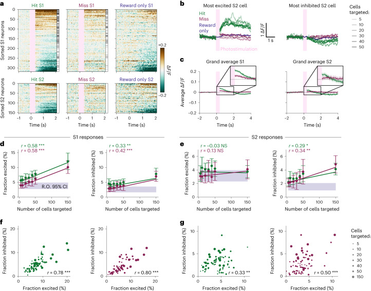
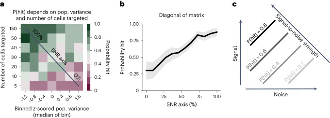
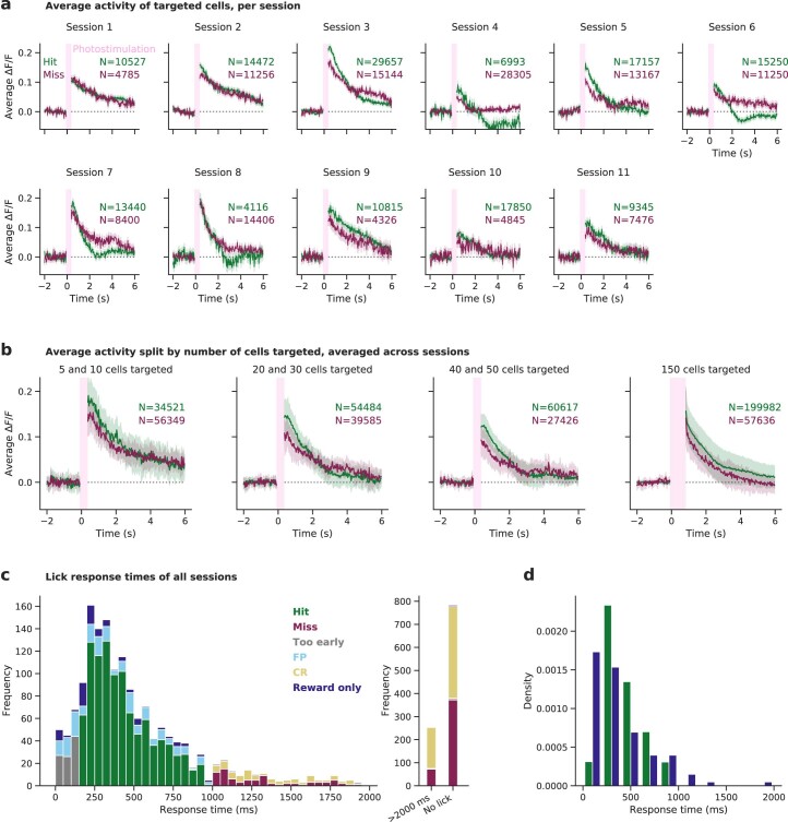
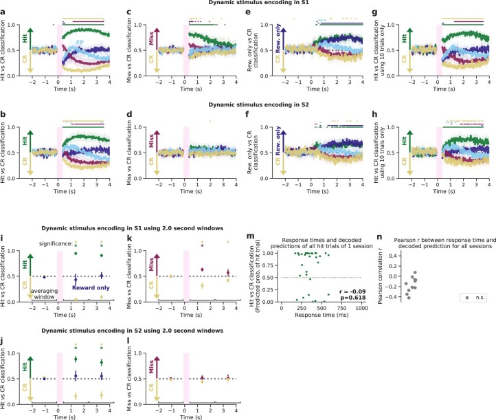
Brains are composed of anatomically and functionally distinct regions performing specialized tasks, but regions do not operate in isolation. Orchestration of complex behaviors requires communication between brain regions, but how neural dynamics are organized to facilitate reliable transmission is not well understood. Here we studied this process directly by generating neural activity that propagates between brain regions and drives behavior, assessing how neural populations in sensory cortex cooperate to transmit information. We achieved this by imaging two densely interconnected regions-the primary and secondary somatosensory cortex (S1 and S2)-in mice while performing two-photon photostimulation of S1 neurons and assigning behavioral salience to the photostimulation. We found that the probability of perception is determined not only by the strength of the photostimulation but also by the variability of S1 neural activity. Therefore, maximizing the signal-to-noise ratio of the stimulus representation in cortex relative to the noise or variability is critical to facilitate activity propagation and perception.

Fig. 1. Recording neural activity in S1 and S2 during behavioral report of targeted 2P photostimulation of S1.

a, Schematic of experimental setup. Left: viral strategy for expression of GCaMP6s and C1V1-Kv2.1-mScarlet in S1 and S2. Right: mice with a cranial window installed over S1 and S2 were head fixed under a 2P microscope. A lick spout was placed within reach of the tongue, through which the animal reported perception of photostimulation by licking and received a water reward. This figure was adapted with permission from Ethan Tyler and Lex Kravitz (Scidraw.io, 10.5281/zenodo.3925901) and Jason Keller (Scidraw.io, 10.5281/zenodo.3925969). b, Example imaging field of view used to localize S1 and S2 by whisker stimulation (stimulus-triggered average wide-field calcium whisker response shown in yellow; see Extended Data Fig. 1 for multiple whiskers), overlaid with aligned 2P images of GCaMP6s (green) and C1V1-Kv2.1-mScarlet (magenta) expression. c, Example 2P calcium imaging field of view with photostimulation targets. The intensity of each pixel is proportional to the change in fluorescence intensity post-photostimulation compared to pre-photostimulation (stimulus-triggered average; Methods); bright pixels indicate a photostimulation-induced increase in calcium activity. Pixels are color-coded based on whether they were photostimulated simultaneously. Non-targeted cells, including those in S2, are not visible because different cells would respond to repeated stimulation of the same group of targeted cells and were, therefore, averaged out. b and c show data from a representative single recording session. d, Top: example activity responses to photostimulation of a single recording session. Orange shows the response to photostimulation of cells directly targeted with light, averaged across cells and across trials. Light and dark blue show the response of cells not directly targeted in S1 and S2, respectively. Only trials in which photostimulation was delivered were included. Data are blanked while the photostimulation laser was on (pink bar), as this causes a large artifact unrelated to neural activity. Bottom: total ΔF/F activity post-stimulus is shown, as defined by the area under the curve (AUC) of the traces of the top panel, for all 11 recording sessions (mean ± 95% confidence interval across sessions). We tested whether each condition was significantly different from 0 (two-sided Wilcoxon signed-rank test, Bonferroni corrected). e, Top: timing of a single behavioral trial. Bottom left: behavioral response matrix. Bottom right: example lick raster from a single session sorted by number of cells targeted and by time within each bin. Each row of the plot shows the first lick within an individual trial. The color bar shows the outcome of the trial as defined in the behavioral response matrix. f, Psychometric curves showing behavioral performance (d′) as a function of the number of cells targeted by photostimulation. Each gray point is the d′ computed for a given number of cells targeted for an individual session, and each gray line is a logistic function fit for an individual session. The thick black line shows the fit for all data points across all sessions (n = 11 sessions; n = 5 mice). The gray dashed line shows that the 50% point from the fit across all sessions occurs at 22 ± 1 cells targeted.

Fig. 2. Activity driven by targeted 2P photostimulation is propagated from S1 to S2.

a, Raster plots showing the trial-averaged response of different trial types (left: hit, middle: miss, right: reward only) to photostimulation (pink vertical bar: hit/miss) and/or reward (hit/reward only) of individual cells from a single session. (All trial types of all sessions are shown in Supplementary Figs. 1 and 2). Cells are sorted by the sum of their trial-averaged responses across all three trial types (Methods). Clear excitatory and inhibitory responses are elicited in S1 and S2 on hit trials that are not observed on miss trials or reward-only trials. The intensity of the grayscale bar on the right-hand side of the hit and miss rasters is proportional to the number of times each cell was directly targeted by the photostimulation beam, for hit and miss trials separately. Trials in which 150 cells were targeted were removed for display because their stimulation period is longer. Data are bound between −0.2 and +0.2 ΔF/F and blanked during the photostimulation (pink bar). b, Left: the ΔF/F activity traces of the most excited S2 cell (of the session of a) are shown, averaged across stimulus conditions. This S2 cell shows a large response on hit trials (green) but no response on miss trials (red) or reward-only trials (blue). The transparency of the line indicates the number of cells targeted in S1. Trials in which 150 cells were targeted were removed for display. Right: equivalent plot for the most inhibited S2 cell of a. c, The average population response to hit and miss trials across all sessions is shown (shaded areas show 95% confidence interval across trials of all sessions). Traces are averaged across cells, trials and sessions for a given trial type. Trials in which 150 cells were targeted were removed for display. The population responses of all other trial types are shown in Extended Data Fig. 3b,c. d, The neural response in S1 on hit and miss trials depends on the number of cells targeted in S1. Left: the fraction of excited cells (Methods) in S1 maps linearly to the number of cells targeted on both hit and miss trials. Right: the fraction of inhibited cells in S1 maps linearly to the number of cells targeted on both hit and miss trials. For hit and miss trials, data are presented as mean ± s.e.m. The shaded purple bar shows the 95% confidence interval across sessions of the fraction of excited or inhibited cells in S1 on reward-only trials. The linear fit was determined using weighted least squares, where the weights were the inverse variance of the trials that constituted a data point, and subsequently bound between their 25th and 75th percentiles to prevent extreme weight values. P values were computed using a two-sided t-test, where significance is indicated by ***P < 0.001, **P < 0.01, *P < 0.05 or NS (not significant). e, Equivalent panel for S1 responses. Left: There is no relationship between the fraction of excited cells in S2 and the number of cells targeted in S1 on hit trials or miss trials. The shaded purple bar shows the fraction of excited or inhibited cells in S2 on reward-only trials. Right: the fraction of inhibited cells in S2 maps linearly to the number of cells photostimulated in S1 on both hit and miss trials. f, The fraction of cells excited by photostimulation in S1 is highly correlated with the fraction of cells inhibited after photostimulation, both on hit trials (left) and on miss trials (right). The size of the circle indicates the number of cells photostimulated. The Pearson correlation coefficient is denoted by r, with significance indicated as before (two-sided t-test). g, The fraction of cells excited by photostimulation in S2 is correlated with the fraction of cells inhibited after photostimulation, both on hit trials (left) and on miss trials (right).

Fig. 3. Perceived photostimuli elicit persistent activity in both S1 and S2 populations.

a, The strength of trial type decoding in the neural population in S1 was dynamically quantified using logistic regression classifiers. Classifiers were trained on each timeframe individually, with activity of all cells in S1 or S2, and tested on held-out data. b, Classifiers were trained, for each timepoint, on S1 activity to classify hit trials from correct-rejection trials and then tested on held-out hit trials (green), correct-rejection trials (yellow) and reward-only trials (blue). Classifications are presented as mean ± s.e.m. across n = 11 sessions. Colored bars above the traces show timepoints at which classifier performance was significantly different from chance (two-sided Wilcoxon signed-rank test, P < 0.05, Bonferroni corrected; Methods). The classifiers were able to distinguish hit trials from correct-rejection trials with high accuracy for several seconds after photostimulation, implying that activity that arose from perceived stimulation persists in S1. Reward-only trials were not classified as hits, showing that the classifiers were not just trained to decode the neural signature of reward on hit trials. c, Classifiers were trained on S2 activity to distinguish hit trials from correct-rejection trials and then tested on hit trials (green), correct-rejection trials (yellow) and reward-only trials (blue). As above, the classifiers were able to decode hit trials from correct-rejection trials for several seconds after photostimulation, implying that activity that arose from perceived stimulation in S1 is propagated to S2 and persists for several seconds. Reward-only trials were not classified as hits, indicating that the model was not just detecting the neural signature of reward on hit trials. d, Classifiers were trained on S1 activity to classify miss trials from correct-rejection trials and then tested on miss trials (red) and correct-rejection trials (yellow). The classifiers were able to distinguish the two trial types for only for ~1 s after photostimulation. This implies that non-perceived stimuli do not generate persistent activity. e, Classifiers were trained on S2 activity to classify miss trials from correct-rejection trials and then tested on miss trials (red) and correct-rejection trials (yellow). The classifiers were not able to classify miss from correct-rejection trials, indicating that non-perceived stimuli were not robustly propagated from S1 to S2, likely because they were also not encoded in S1 (d). CR, correct-rejection; dim., dimension.

Fig. 4. Pre-stimulus population in S1 predicts the upcoming trial outcome.

a, Illustration of neural activity throughout a trial. Only the activity in the 0.5 s before the stimulus on a given trial is included in subsequent panels. First, we considered two metrics of pre-stimulus neural activity: the population mean and the population variance. b, Comparison of population metrics of pre-stimulus S1 activity before hit trials and before miss trials. Left: no evidence that mean population activity pre-stimulus predicts the upcoming trial outcome. Right: population variance is significantly higher before miss trials than before hit trials. Pre-stimulus population metrics in S1 were computed trial-wise and z-scored across trials within a session before being split into hit and miss trials and averaged across a session. P values were tested for a difference in session-wise population metrics between hit and miss trials (two-sided Wilcoxon signed-rank test). c, The probability of detecting the photostimulation decreased linearly with increasing pre-stimulus population variance in S1 for 10 of 11 sessions (one-sided t-test, Bonferroni corrected). Trials within a session were binned by their z-scored population variance, and this was correlated to the probability of a hit trial within that bin. distr., distribution; pop., population; var., variance.

Fig. 5. Miss trials are preceded by higher effective recurrence.

a, To quantify effective recurrence R in a network, we first apply latent factor analysis to identify activity that is putatively driven by shared external input. We then subtract out this ‘shared’ activity and focus on the remaining ‘non-shared’ activity. b, Variance explained by each of the first five latent factors (miss: red, hit: green). c, The variance explained by the first factor (also called ‘across-neuron population-wise correlation’; Supplementary Methods) is not significantly different between hit and miss trials (two-sided Wilcoxon signed-rank test, P = 0.168). d, For 6.5 s of non-shared pre-trial activity, the cross-neuron correlation matrix is calculated (orange and red stars show the process for a pair of example neurons; gray box highlights that of a single pair; yellow triangle marks the off-diagonal entries that are analyzed further). e, The mean off-diagonal cross-correlation is not significantly different before hit or miss trials (P = 0.37, two-sided Wilcoxon signed-rank test). f, Cross-covariance matrix of the non-shared activity (yellow triangle marks the off-diagonal entries used to compute recurrence). g, Histogram of the cross-covariance matrix; gray arrows indicate the variance of the distribution σ_CC. h, The relationship between σ_CC and the effective recurrence R of the local network is known from theoretical derivations (Methods; plotted in black for a network of 50,000 neurons). Data for individual sessions are shown as gold and silver circles (S1 and S2, respectively); straight lines show the average across sessions; and dotted lines show the spread (mean ± s.d.). i, The effective recurrence R before stimulation is significantly different on hit and miss trials, suggesting that lower recurrence facilitates stimulus detection (P = 0.002, two-sided Wilcoxon signed-rank test). j, The average photostimulation response of the targeted cells on either hit or miss trials (excluding trials where 150 targets were stimulated, averaged across sessions in bold and averaged per session in shade). k, The ‘network response timescale’ τ_post was determined by fitting an exponential decay function per session. l, The inferred τ_post values (yellow circles) were better explained by the linear network theory (gray line, r² = 0.44) than a simple linear regression (not shown, r² = 0.38). m, The inferred network response timescale τ_post is significantly different on hit and miss trials (P = 0.023, two-sided Wilcoxon signed-rank test). expl., explained.

Fig. 6. Stimulus strength and neural population variance underpin perception.

a, The interaction between pre-stimulus population variance in S1 and the number of cells targeted by photostimulation defines the probability of a hit trial. Trials were binned by their z-scored population variance and by the number of cells targeted; the probability of a hit within each bin is plotted on a two-dimensional axis, pooled across all sessions. Increasing the number of cells targeted (that is, signal strength) and decreasing the pre-stimulus variance (that is, ‘noise’) generally yielded a greater probability of a hit trial. This is referred to as the SNR, as indicated by the diagonal black arrow. b, Maximizing the SNR of the stimulus resulted in the maximal probability of a hit trial. Data as in a but projected onto the SNR axis—as indicated in a—by averaging across all bins that project orthogonally onto each point on this axis. Data are presented as mean ± s.e.m. c, Schematic outlining the intuition for the SNR axis. Increasing the number of cells targeted on a given trial maximizes the signal of that stimulus. Noise is proportional to the population variance as there is more excitation and suppression from baseline in a population with high variance. The probability of hit is maximal when SNR is maximal, as the stimulus is more likely to be detected above ongoing activity.

Extended Data Fig. 1. Mapping whisker S1 and S2 regions using widefield calcium imaging and whisker stimulation.

(a) Single whiskers were deflected one at a time by threading them on to a capillary tube attached to a piezoelectric actuator. This figure was adapted with permission from Ethan Tyler and Lex Kravitz (10.5281/zenodo.3925901). (b) Each whisker was deflected multiple times and the results were averaged. The stimulus-triggered average responses from all whisker deflections is plotted on an image of the cerebral vasculature. (c) Individual stimulus-triggered average images from each whisker shows the topographical organisation of the barrel cortex in whisker S1 and the mirrored topography in whisker S2. Panels b) and c) show data from a representative single recording session.

Extended Data Fig. 2. Activation of targeted cells by photostimulation.

(a) The average ΔF/F activity of the cells targeted by photostimulation is shown (mean values +/− SEM) per recording session, for Hit and Miss trials separately. Targeted cells are activated similarly, with the notable exception of Hit-only inhibition at ~2 seconds post-stimulus in 3 recording sessions (of the same animal), indicating that the photostimulation-induced activation is largely independent of behavioural outcome. All trials with 5 to 50 cells targeted were used; trials where 150 cells were targeted were excluded because almost all of these trials resulted in a Hit outcome, biasing the averages. (b) The same data as panel a) is shown, but now averaged across animals and split by number of cells targeted (mean values +/− SEM). (c) Stacked histogram of the animals’ response times (defined by the time of the first lick) for each trial type. All trials with a response time within 2000 ms of all recording sessions are shown in the left panel, while trials with a response time greater than 2000 ms and trials where no lick occurred are grouped in the right panel. (d) Density histograms of response times of hit and reward only trials. Same data as in panel a), but normalised per trial type and binned per 200 ms. Medians (248 ms for reward only trials and 383 ms for hit trials) are significantly different (p = 0.01, (two-sided) Mood’s median test).

Extended Data Fig. 3. Fraction of cells responding and grand average traces of all trial types in S1 and S2.

(a) The fraction of responsive cells (both excited and inhibited) on each trial type across all numbers of cells targeted. One-sided Wilcoxon signed-rank tests were used to test whether the fraction of responsive cells of hit trials was significantly greater than on other trial types (Bonferroni corrected for 8 tests). N = 11 independent recording experiments. Boxplots are defined by the median (centre), interquartile range (IQR) box, 1,5 IQR whiskers plus any outliers. (b) Average population responses of all trial types across all sessions. Traces are averaged across cells, trials and sessions for a given trial type. Trials in which 150 cells were targeted were removed for display (and shown in c). The time course of reward only trials is different from the time course of hit trials, hinting that the neural activity on hit trials constitutes more than motor preparation, movement, and reward related activity. This is further quantified in Figs. 2, 3. (c) As above but showing exclusively trials in which 150 cells were targeted.

Extended Data Fig. 4. Dynamic decoders of all trial types.

The strength of stimulus decoding of trial type in the neural population in S1 was dynamically quantified using logistic regression models. Models were trained on each time frame individually, with activity of all cells in S1 or S2, and tested on held-out data. (a) Models were trained, for each time point, on S1 activity to classify hit trials from correct rejection trials and then tested on held-out hit trials (green), correct rejection trials (yellow), reward only trials (dark blue), false positive trials (light blue) and miss trials (red). Classifications are presented as mean values +/− SEM across N = 11 sessions in panels (a)-(l). Coloured bars above the traces show time points at which classifier performance was significantly different from chance (two-sided Wilcoxon signed-rank tests, p < 0.05, Bonferroni corrected, see Methods). (b) As above, but trained on S2 activity. (c) Models were trained on S1 activity to classify miss trials from correct rejection trials and then tested on miss trials (red), correct rejection trials (yellow) reward only trials (dark blue), false positive trials (light blue) and hit trials (green). (d) As above, but trained on S2 activity. (e) Models were trained on S1 activity to classify reward only trials from correct rejection trials and then tested on reward only (dark blue), correct rejection trials (yellow), miss trials (red), false positive trials (light blue) and hit trials (green). (f) As above, but trained on S2 activity. (g) As (a) but the number of trials was restricted to 10 for each type, matching the total number of reward only trials recorded. (h) As (b) but the number of trials was restricted to 10 for each type, matching the total number of reward only trials recorded. (i-l) Equivalent to Fig. 3, but now using 2-second windows to train the classifiers. Three windows were used (−2.0 s up to and including −0.1 s, 0.4 s u/i 2.3 s, 2.4 s u/i 4.3 s), shown at the bottom of each panel. For each window, neural activity was averaged across time, per neuron per trial. Classifiers were then trained and evaluated as before and described in Methods. Asterisks indicate significant differences with chance level accuracy 0.5 (two-sided Wilcoxon signed-rank test, bonferroni-corrected p value < 0.05). As in panels (a)-(h), classifications are presented as mean values +/− SEM across N = 11 sessions in panels. (m) Comparison between lick response time and predicted outcome for all hit trials in S2. We considered the first decoder post-stimulus (at t = 367 ms), and compared for each trial the predicted outcome evaluated on withheld test data to the response time. This panel shows one example session (same session as Fig. 2a), and its Pearson correlation value r and associated (two-sided) p value. (n) Pearson correlation values r between response time and decoded S2 predictions of hit trials of all 11 sessions are shown. A Bonferroni multiple-comparison correction of N = 11 (sessions) was used.

Extended Data Fig. 5. Dynamic decoders of individual sessions.

(a–d) As Fig. 3, but displaying classifier performance for each individual session. Traces were smoothed using a running mean of 5 time points for visual clarity.

Extended Data Fig. 6. Further population metrics of pre-stimulus activity.

Comparison of population metrics of pre-stimulus in S1 (a) and S2 (b) activity prior to hit trials and prior to miss trials. The first two panels show the two metrics of Fig. 4b. Next, two other significant task variables are shown; the trial number (an integer between 0 and the total number of trials in a session, indicating the number of trials previously undertaken by the animal in a given session) and the reward history (defined as % hit trials in the 5 preceding photostimulated trials). All variables were z-scored for clarity, and significance was assessed using two-sided Wilcoxon signed-rank tests. (c, d) The co-variability of the significant statistics of panels a and b was assessed using Pearson correlation (two-sided t-test). In sum, as recording sessions progress, reward history declines, and population variance is correlated to this trend. (e) Population variance is significantly correlated between S1 and S2 on a single-trial level (two-sided t-test). (f) Population variance is significantly correlated to the population mean on a trial-by-trial basis in both S1 and S2 (two-sided t-test). Population mean and variance were z-scored in all panels to allow comparison between different recording sessions. Trial number and reward history were z-scored in panels a-b only.

Extended Data Fig. 7. Dynamic decoding results split by population variance.

(a–d) The decoders of Fig. 3 are shown, but additionally split by population variance. In other words, this figure shows the same data, but with an additional condition to separate trials by. Each recording session was split into 3 tertiles of equal size based on population variance (that is 3 bins were used), which were then averaged across sessions. Classifications are presented as mean values +/− SEM across N = 11 sessions. (e-h) The decoders of Fig. 3 are shown, but additionally split by number of cells targeted. Three ‘number of cells targeted’ conditions were used (instead of six) to increase data size, in particular for the rare scenarios (such as, for example, ‘Miss 40-50’). Two recorded sessions did not include data for one trial type/cells targeted combination, and were therefore omitted (for that combination only). Hence, classifications are presented as mean values +/− SEM across N = 9 sessions.

Extended Data Fig. 8. Recurrence analysis for all, shared and non-shared activity.

The recurrence analysis results of Fig. 5 are shown in more detail. The first row (a-c) shows the mean off-diagonal correlation: for (a) all activity, (b) shared activity, and (c) non-shared activity. The second row (d–f) shows the mean on-diagonal covariance μ_V. The third row (g–i) shows the standard deviation of the off-diagonal covariance σ_CC. The fourth row (j–l) shows the ratio of the standard deviation of the off-diagonal covariance and the mean on-diagonal covariance σ_CC/μ_V. The fifth row (m–o) shows the change in recurrence R. The sixth row (p–r) also shows the change in the recurrence R, but estimated from neural activity in S2 instead of in S1. P values tested for a difference in session-wise population metrics between hit and miss trials (two-sided Wilcoxon signed-rank test without correction multiple comparison).

Extended Data Fig. 9. Recurrence analysis for different number of latent factors.

The stability of the results shown in Fig. 5 with respect to the choice of the number of latent factors is explored (dashed vertical line denotes the 5 latent factors we used in Fig. 5). The first row (a, b) explores the hit-miss difference for the mean off-diagonal correlation; shown are (a) the effect size (dashed horizontal line denotes nil effect) and (b) the p-value of the observed effect (dashed horizontal lines denote p = 0.05, p = 0.01, and p = 0.001; two-sided Wilcoxon signed-rank test without correction multiple comparison), for all activity (black diamond), shared activity (purple crosses) and non-shared activity (pink crosses). The second row (c, d) explores the hit-miss difference for the mean on-diagonal covariance μ_V. The third row (e, f) explores the hit-miss difference for the standard deviation of the off-diagonal covariance σ_CC. The fourth row (g, h) explores the hit-miss difference for the ratio of the standard deviation of the off-diagonal covariance and the mean on-diagonal covariance σ_CC/μ_V. The fourth row (i, j) explores the hit-miss difference for the recurrence R. The fifth row (k, l) shows the same hit-miss difference for R, but uses Principal Component Analysis (PCA) instead of LFA to estimate shared activity.

Extended Data Fig. 10. Pre-stimulus pupil size does not influence trial outcome.

(a) Pupil size was measured for 3 sessions (sessions 7, 8 and 9, corresponding to Supplementary Fig. 2), see Methods. (b) Trial- and session-averaged pupil size dynamics for hit and miss trials, where shaded areas indicate the 95% confidence interval of the mean (across sessions and trials). The time-averaged pre-stimulus pupil size was not significantly different between hit and miss trials (two-sided t-test). (c) Population variance was very weakly correlated to pupil size across all sessions (both averaged across 500 ms pre-stimulus per trial) (two-sided Pearon correlation r = 0.12, p = 0.02). (d–f) Trial-averaged pupil size dynamics per session, where shaded areas indicate the 95% confidence interval of the mean (across trials). Pre-stimulus differences between hit and miss were not significant for any of the sessions (two-sided t-tests), although session 7 (panel d) almost reached the significance threshold (p = 0.053). (g–i) Population variance vs pupil size per session. Two-sided Pearson’ correlation was significant for only one of the sessions (session 7).

References

1. Stringer C, et al. Spontaneous behaviors drive multidimensional, brainwide activity. Science. 2019;364:255. - PMC - PubMed
1. Mante V, Sussillo D, Shenoy KV, Newsome WT. Context-dependent computation by recurrent dynamics in prefrontal cortex. Nature. 2013;503:78–84. - PMC - PubMed
1. Simons DJ. Response properties of vibrissa units in rat SI somatosensory neocortex. J. Neurophysiol. 1978;41:798–820. - PubMed
1. Stringer C, Pachitariu M, Steinmetz N, Carandini M, Harris KD. High-dimensional geometry of population responses in visual cortex. Nature. 2019;571:361–365. - PMC - PubMed
1. Yang T, Shadlen MN. Probabilistic reasoning by neurons. Nature. 2007;447:1075–1080. - PubMed
Publication types