Environmental gradients reveal stress hubs pre-dating plant terrestrialization

Abstract

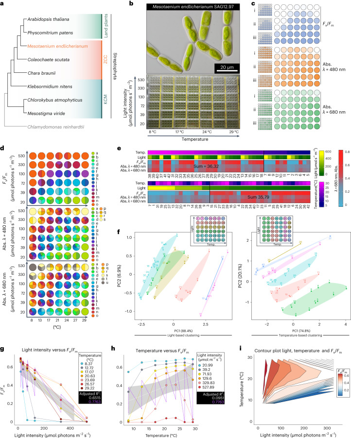
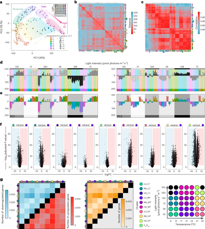
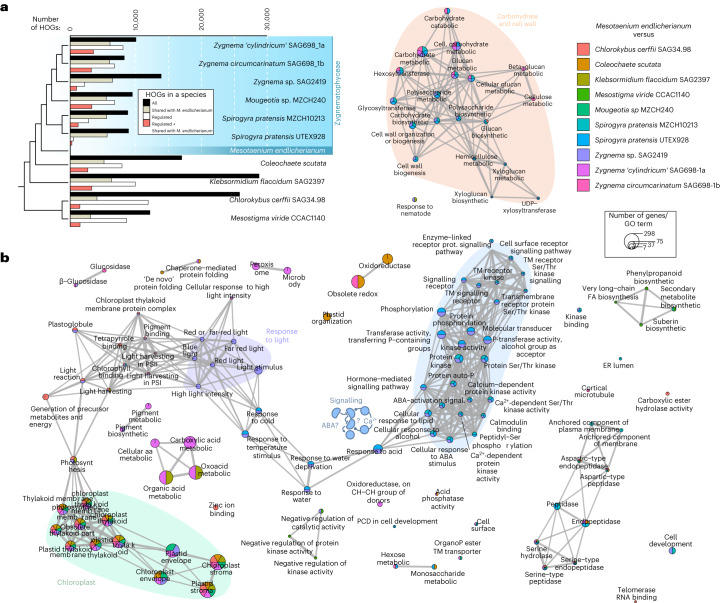
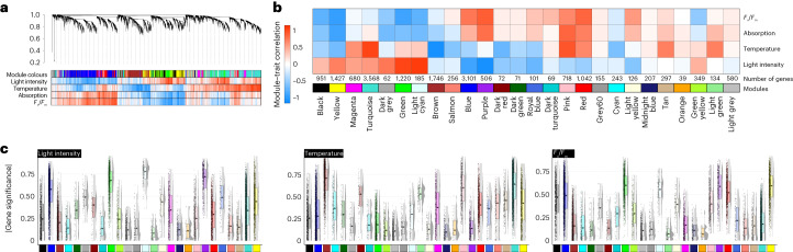
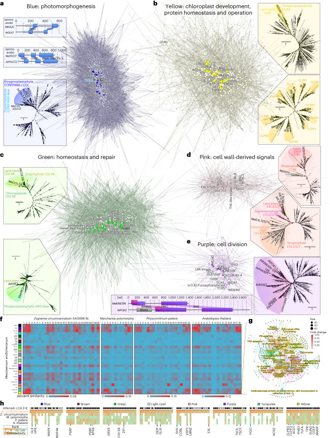
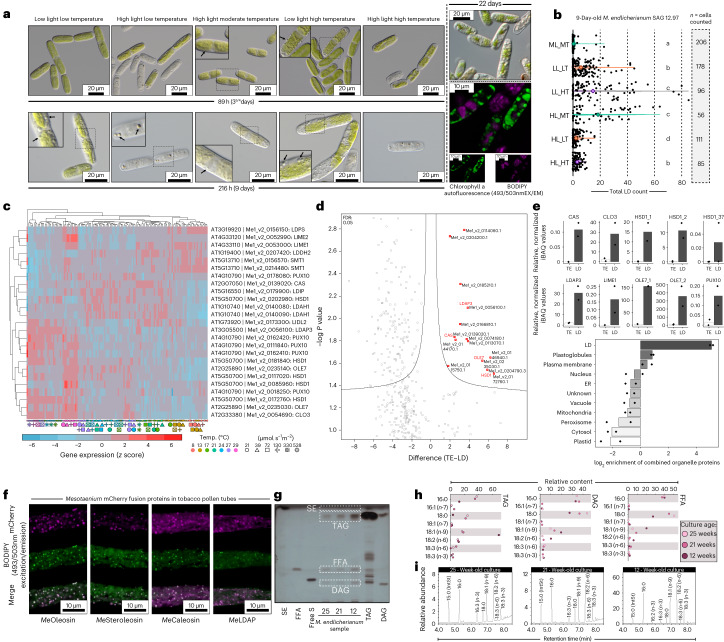
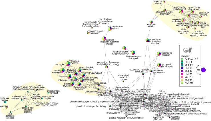
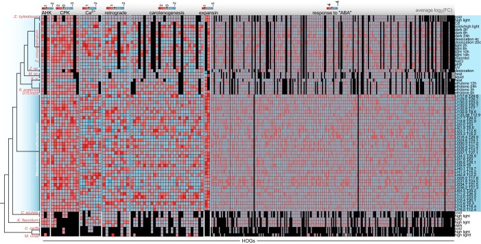
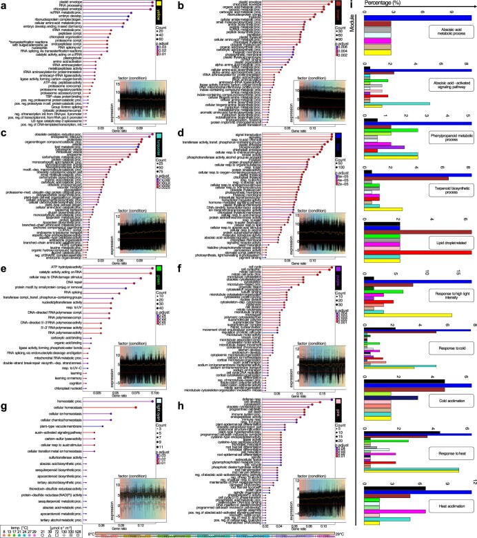
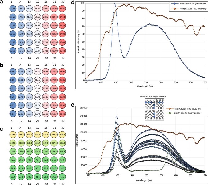
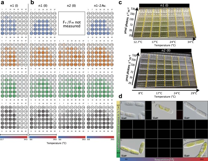
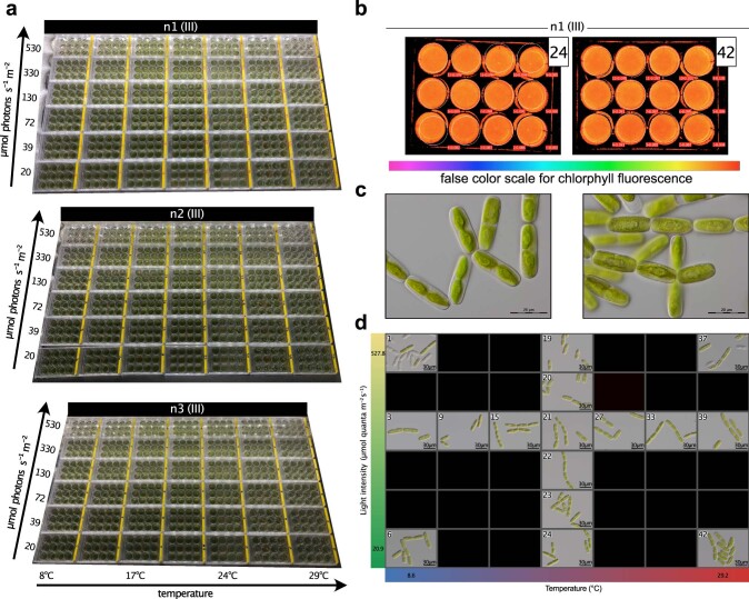
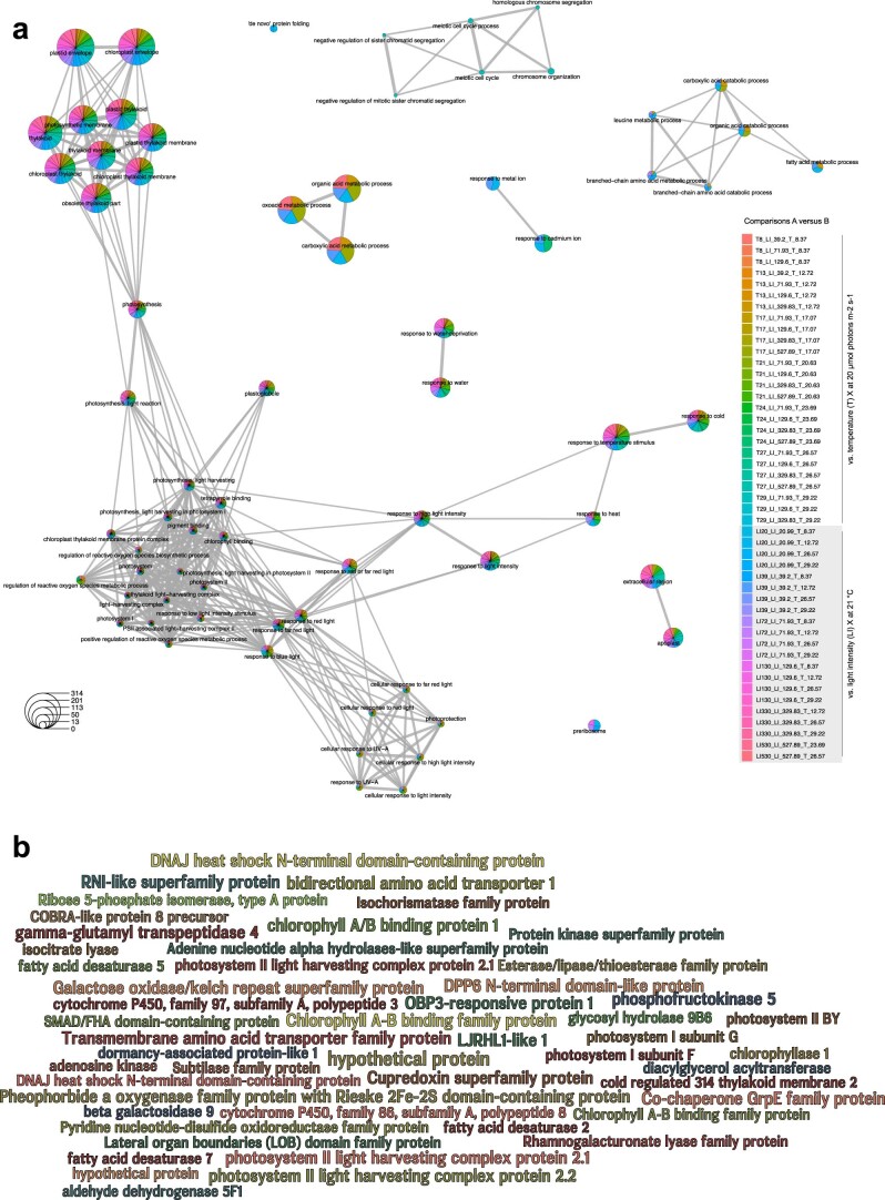
Plant terrestrialization brought forth the land plants (embryophytes). Embryophytes account for most of the biomass on land and evolved from streptophyte algae in a singular event. Recent advances have unravelled the first full genomes of the closest algal relatives of land plants; among the first such species was Mesotaenium endlicherianum. Here we used fine-combed RNA sequencing in tandem with a photophysiological assessment on Mesotaenium exposed to a continuous range of temperature and light cues. Our data establish a grid of 42 different conditions, resulting in 128 transcriptomes and ~1.5 Tbp (~9.9 billion reads) of data to study the combinatory effects of stress response using clustering along gradients. Mesotaenium shares with land plants major hubs in genetic networks underpinning stress response and acclimation. Our data suggest that lipid droplet formation and plastid and cell wall-derived signals have denominated molecular programmes since more than 600 million years of streptophyte evolution-before plants made their first steps on land.

Fig. 1. A fine-combed setup for assessing environmental responses in Mesotaenium.

a, Cladogram of Streptophyta, highlighting that Mesotaenium endlicherianum SAG 12.97 is a representative of the closest algal relatives of land plants. KCM, the grade of Klebsormidiophyceae, Chlorokybophyceae and Mesostigmatophyceae; ZCC, the grade of Zygnematophyceae, Coleochaetophyceae and Charophyceae. b, M. endlicherianum grown in C-medium in 42 12-well plates on a gradient table that produces a temperature range of 8.6 ± 0.5 °C to 29.2 ± 0.5 °C on the x axis and an irradiance gradient of 21.0 ± 2.0 to 527.9 ± 14.0 µmol photons m⁻² s⁻¹ on the y axis; for phenotyping per well, at least ten micrographs were taken, all showing similar phenotypes of the cells. c, Overview of the measured maximum quantum yield F_v/F_m as a proxy for gross physiology (blue) and absorption (abs.) at 480 (orange) and 680 nm (green); individual replicates of the biological triplicates are shown on the left and the average values are shown on the right. d, Statistical analysis of the physiological values (F_v/F_m, abs. 480 nm, abs. 680 nm). Numbers correspond to environmental conditions on the table. Biological triplicates were grouped into significant groups (a–o, a–s and a–u) with R (version 4.1.3) using a Kruskal–Wallis test coupled with Fisher’s least significance; P values were Bonferroni corrected. Significant differences at P ≤ 0.001 are shown as letters. e, Heat maps displaying averaged physiological values of the 42 conditions sorted either by temperature (temp.) or light. A cut-off was set (black vertical line) on the basis of the distribution of the highest values, which were then summed to determine a positive correlation with temperature or light conditions. f, Two PCAs showing the correlation of light conditions (left) or temperature conditions (right) to physiological values (F_v/F_m, abs. 480, 680 nm). Clusters are shown in different colours, which are also visualized in an overview scheme of the gradient table at the top of the plots. g,h, Unifactorial regression analysis of light intensity (g) and temperature (h) versus F_v/F_m; note the unifactorial linear regression curves (white) versus the bifactorial (violet). i, Contour plot of the bifactorial impact of light and temperature on F_v/F_m (gradient colour).

Fig. 2. Global profiles of environment-governed gene expression response.

a, PCA visualizing PC1 and PC2. Backgrounds were drawn to highlight our interpretation of the observed trends; samples are coded by colour (temperature) and symbols (irradiance in µmol photons m⁻² s⁻¹). Samples that did not yield usable RNA are indicated as grey dots in the top-right overview of the experimental setup. b, Visualization of Euclidean distances between samples via heat map, from red, zero distance, to blue, furthest distance (a distance of 300). c, Heat map of Spearman correlation between samples, from red, maximum correlation (1.0), to blue, least correlation (<0.8). The clusters were calculated via the Euclidean distance. d,e, PC1 and PC2 scrutinized using a small multiples method of light intensity (d) and temperature (e). In d, shades of grey correspond to different light intensities. In e, different colours represent different temperatures and were mapped with the same colours as a. To perform differential gene expression analysis, we divided the table into nine sectors (see scheme of the table); additionally, a tenth group was raised based on F_v/F_m < 0.5. Linear models were fitted for each gene and empirical Bayes statistics computed for DEGs by the limma package. In total, 37 comparisons were made. DEGs were defined as genes with an absolute fold change (FC) ≥2 and Benjamini–Hochberg-adjusted P value less than 0.01. f, Volcano plots of DEGs for nine selected comparisons based on the sectors and the F_v/F_m < 0.5 criterion. g, Heat maps of numbers of DEGs for all sector-based comparisons (blue, downregulation; red, upregulation; yellow, sum of up- and downregulated genes); grey bars label the first component (treatment) for calculating the contrasts (treatment versus control).

Fig. 3. Comparative analyses of global differential gene expression profiles across stress-treated streptophyte algae.

Publicly available data on stress transcriptomes from ten different streptophyte algae were downloaded and significant differential gene expression between stress treatment and control per species were calculated. Phylogenetic HOGs were inferred with Orthofinder. a, Bar graph of the number of all HOGs detected (black), HOGs shared with Mesotaenium endlicherianum (tan), all regulated HOGs in a given species (white) and, of those regulated, which are in the same HOG as significantly regulated genes in Mesotaenium (red); the relationship between the streptophyte algae is shown by the cladogram on the left. b, GO term-based biological theme comparison of these shared significantly regulated genes in HOGs. Note the recurrent pattern of chloroplast-associated differential gene expression (green), light quality (purple) and the putative integration of calcium signalling with pathways known from phytohormone signalling, including ABA, in land plants (blue, also note the little sketch of a hypothetical model). PCD, programmed cell death.

Fig. 4. Unsupervised gene expression clusters recover genetic programmes separated by environmental cues.

Gene expression clustering into 26 coloured modules was performed using WGCNA; grey is the module of unclustered genes. a, Hierarchical cluster tree of 17,095 genes. The heat map below the dendrogram and module colour assignment shows the gene significance measure (from red, positive correlation, to white, no correlation, to blue, negative correlation) for the four different conditions or physiological parameters. b, Heat map of the module–trait correlation based on eigengenes (from red, positive correlation, to white, no correlation, to blue, negative correlation); see Supplementary Fig. 7. c, Box plots of the mean gene significance across modules (given in the corresponding module colour) towards the parameters light intensity, temperature and F_v/F_m. The box plots display the interquartile range (IQR) of the data, compactly displaying the distribution of a continuous variable. They visualize five summary statistics (the median, two hinges and two whiskers). The upper whiskers extends from the hinges to the largest/smallest value no further than 1.5× IQR from the hinge. Each data point (n) is a gene, and the total n of genes is the same as shown in b. We calculated the gene significance for each gene using the WGCNA package and Pearson method.

Fig. 5. Molecular programmes for environmental responses around recurrent plant hubs.

a–e, Visualization of the co-expression networks clustered by WGCNA into the modules blue (3,101) (a), yellow (1,427) (b), green (1,220) (c), pink (718) (d) and purple (506 genes) (e). Nodes (circles) represent genes connected by edges whose weight (light to dark colour) is based on a weighted TOM. Brightly coloured nodes represent the 20 most connected genes (hubs) and are annotated based on homology; all other nodes are depicted in the corresponding paler colour. Around the clusters, different protein-coding hub genes are highlighted, giving information such as predicted domain structures or phylogenetic relationships; for fully labelled phylogenies, see Supplementary Fig. 26b. Circles in phylogenies give a scale of the ultrafast bootstrap support values; diamonds indicate high (>90%) support for branches separating highlighted clades. An alignment of GLK homologues can be found in Supplementary Fig. 8. f, Using WGCNA, co-expression networks were computed from 212 publicly available RNA-seq datasets from Z. circumcarinatum, M. polymorpha, P. patens and A. thaliana exposed to diverse abiotic challenges, yielding between 12 and 29 modules (labelled above the heat map), and orthogroups for all genes in the modules of these different species were determined. The heat map shows the similarity, based on Jaccard indices, between the modules of Mesotaenium (same colours as throughout the paper, see Fig. 4b) and the co-expression modules in the three land plants as well as Zygnema; red to blue colour gradients indicate high to low Jaccard similarity. g, Cnet plot of the enriched GO terms in the module ‘Arabidopsis 18’, which has high Jaccard similarity to the M. endlicherianum module yellow—note the recurrent terms of plastid operation and, especially, the Clp complex. h, Heat map of the connectivity ranks across all five species for homologues of hub genes of Mesotaenium, from orange (high) to green (low connectivity). Black boxes (top row) indicate if our phylogenies (see data on Zenodo) suggest that the hub genes fall into families that were present in the last common ancestor of Zygnematophyceae and land plants, and hence emerged before plant terrestrialization; white boxes signify the absence of such indication and grey boxes highlight ambiguous relationships.

Fig. 6. LDs accumulate in Mesotaenium upon changing environments.

a, DIC and confocal micrographs of Mesotaenium endlicherianum SAG 12.97 cells accumulating LDs (arrows) upon exposure to different temperature/light conditions (abbreviations) of the gradient table for 89 h or 216 h. For confocal microscopy, algae were cultured independent of table conditions at 75 µmol photons m⁻² s⁻¹ and 22 °C for 22 days. LDs are visible as distinct globular structures and were stained with BODIPY (false-coloured green; 493 nm excitation, 503 nm emission); chlorophyll autofluorescence in false-coloured purple; for each condition, at least ten micrographs were taken, all showing similar phenotypes of the cells. b, Violin plots of LD quantification after 9 days of exposure to different environmental conditions; significance grouping (Mann–Whitney U) is based on P < 0.05; see also Supplementary Fig. 27. c, Heat map of row-scaled z scores of the expression of homologues for LD biogenesis and function (see also Supplementary Fig. 28). Conditions are displayed at the bottom as symbols in different colours; best Arabidopsis hits (via BLASTp) are shown on the right. d,e, Proteomic investigation into lipid-enriched phases extracted from Mesotaenium; note the enrichment in hallmark proteins of LDs. Volcano plot showing significantly (false discovery rate (FDR) <0.05) enriched Mesotaenium proteins in the lipid-enriched (LD) versus the TE (d). Bar plots show the relative, normalized iBAQ values for ten LD signature proteins detected in Mesotaenium (e). Bottom bar plot shows the log₂ enrichment of proteins characteristic for subcellular compartments. LL, ML and HL, low, moderate and high light; LT, MT and HT, low, moderate and high temperature, respectively; ER, endoplasmic reticulum. f, LD proteins of M. endlicherianum localize to LDs in tobacco pollen tubes: cLSM images of transiently expressed proteins appended to mCherry in transiently transformed N. tabacum pollen tubes. LDs were stained with BODIPY 493/503; for each construct, the images are representative of at least nine micrographs of transformed pollen tubes per fusion construct. Scale bars, 10 µm. g,h, Lipid composition in M. endlicherianum LDs of 12- to 25-week-old cultures and standards for sterol esters (SE), FFA, free sterols (free S), TAG and DAG via analytical TLC (g) and preparative TLC followed by GC for profiling (h). i, Full lipid profiles assessed via GC. Source data

Extended Data Fig. 1. Biological theme comparison summarizing all GO term enrichment analysis with adjusted p value ≤ 0.01 of DEGs against all genes that were expressed and passed the filtering in our analyses as background.

The size of each circle is proportional to the count of each GO-term. Only the top 30 enriched terms are shown.

Extended Data Fig. 2. Heat maps of average differential gene expression in log₂(fold change) per HOG.

From the strongest upregulation in red to the strongest downregulation in blue; black means that no HOG was found. The heat maps were sorted by phylogeny (see the cladogram on the left) and treatment (written on the right); light teal highlights the data on Zygnematophyceae, dark teal on Mesotaenium endlicherianum.

Extended Data Fig. 3

Enriched GO-terms for eight of the 26 modules; each inset shows the gene expression profiles of all genes in a given module. (a–i) Arabidopsis homologs for key processes were mined based on keywords; they were retrieved from a look-up table of BLASTp hits in a search of Mesotaenium V2 against A. thaliana representative protein sequences. Bar charts show the percentage of detected Mesotaenium homologs across the modules relative to the number of all Arabidopsis IDs assigned to the terms. No BLAST hit was not depicted. Abbreviations: proc. = process; reg. = regulation; biogen. = biogenesis; develop. = development; pos. = positive; neg. = negative; init. = initiation; GEP = Gene expression profile; med. = mediated; dep. = dependent; modif. = modification; conjug. = conjugation; anneal. = annealing; compl. = complex; synth. = synthesis; resp. = response; transf. = transferring.

Extended Data Fig. 4. Pre-experimental setups: temperature conditions comparison, light intensities, and light spectra.

(a) Temperature conditions for the first experimental setup (n1(I)) depicted by a blue to red color gradient (see also supplementary table ST 1.4). (b) Temperature conditions for the second and the final experimental setup (n1(II), n2(II), n1(III), n2(III), and n3(III)) depicted by a blue to red color gradient (see also supplementary table ST 1.2). (c) Light intensity/irradiance values depicted by a green to yellow color gradient (see also supplementary table ST 1.1). (d) Average light spectra of the gradient table (blue) assessed using SpectraPen (PSI, Brno, CZ) compared to a spectra assessed of natural sunlight (orange). (e) Light spectra of various plates of the gradient table (see overview) in various shades of blue assessed using SpectraPen (PSI, Brno, CZ) compared to a light spectrum assessed of natural sunlight (orange) and a light spectrum from a growth lamp used for flowering plants.

Extended Data Fig. 5. Pre-experimental setup II: Fv/Fm, absorption, and morphology.

(a) Fv/Fm values (blue gradient) and absorption values (orange, green, grey color gradient, Colors indicate measured wavelength: orange gradients = Absorption measured at λ 480 nm, green gradients = Absorption measured at λ 680 nm, grey gradients = Absorption measured at λ 750 nm) of the first pre-experimental setup (n1(I)) with temperature settings ranging from 12.7–34 °C. (b) Fv/Fm and absorption values of second pre- experimental setup (n1(II) and n2(II)) and averaged values (n1-2 Av.) with new temperature settings ranging from 8.6 -29.0 °C. (c) Photographs of the pre-experimental setups n1(I) with temperature conditions ranging from 12.7–34 °C and n2(II) with temperature conditions ranging from 8.6 to 29.0 °C after incubation on the table for 216 h (n1(I)) or 191 h (n2(II)) respectively. The photograph of pre-experiment n2(I) is not shown. (d) Differential interference contrast (DIC) micrographs of SAG 12.97 cells (pre-experimental setup n1(II)) under most extreme environmental conditions (four corners: samples 1, 6, 37, and 42) as well as under high irradiance 527.8 µmol photons m^-2 s^-1 at 20.5 °C; for each well, at least 10 micrographs were taken, all showing similar phenotypes of the cells.

Extended Data Fig. 6. Main-experimental setup (n1,2,3 (III)): Morphology and growth.

(a) Photographs of the main experimental setups n1, n2, and n3 (III) with temperature conditions ranging from 8.6 to 29.0 °C after incubation on the table for 65 h. (b) Fm measurements (maximal fluorescence) using IMAGING-PAM in various table conditions, legend on the right is a false color gradient indicating fluorescence intensity. (c) Differential interference contrast (DIC) micrographs of SAG12.97 cells grown on C-Medium (growth conditions see methods: growth conditions prior to exposure to environmental conditions); at least 10 micrographs were taken, all showing similar phenotypes of the cells. (d) Differential interference contrast (DIC) micrographs of SAG12.97 under most extreme environmental conditions (four corners: samples 1, 6, 37, and 42) as well as along an irradiance gradient at 21 °C (samples 19–24) and a temperature gradient at 130 µmol photons m^-2 s^-1 (samples 3, 9, 15, 21, 27, 33, and 39); for each well, at least 10 micrographs were taken, all showing similar phenotypes of the cells.

Extended Data Fig. 7. Differential gene expression comparisons highlight plastid-related responses.

(a) Biological theme comparison of GO terms enriched in differential gene expression analyses in which one factor was always kept constant; the top 10 different connected graphs are shown. (b) Wordle of the 124 genes that showed significant regulation across multiple comparisons shown in main Fig. 2f,g and Extended Data Fig. 1; word size correspond to the number of comparisons in which a gene appeared. Color serves to increase the contrast between words.

Extended Data Fig. 8. Module stability analysis.

We performed 200 simulations by sampling from our input expression profiles under different conditions using the WGCNA package. Each row in the heat map represents a simulation and stable modules form a ‘column’ of similar color on the heat map.

References

1. Bar-On YM, Phillips R, Milo R. The biomass distribution on Earth. Proc. Natl Acad. Sci. USA. 2018;115:6506–6511. doi: 10.1073/pnas.1711842115. - DOI - PMC - PubMed
1. Lenton TM, et al. Earliest land plants created modern levels of atmospheric oxygen. Proc. Natl Acad. Sci. USA. 2016;113:9704–9709. doi: 10.1073/pnas.1604787113. - DOI - PMC - PubMed
1. Wodniok S, et al. Origin of land plants: do conjugating green algae hold the key? BMC Evol. Biol. 2011;11:104. doi: 10.1186/1471-2148-11-104. - DOI - PMC - PubMed
1. Wickett NJ, et al. Phylotranscriptomic analysis of the origin and early diversification of land plants. Proc. Natl Acad. Sci. USA. 2014;111:E4859–E4868. doi: 10.1073/pnas.1323926111. - DOI - PMC - PubMed
1. Puttick MN, et al. The interrelationships of land plants and the nature of the ancestral embryophyte. Curr. Biol. 2018;28:733–745. doi: 10.1016/j.cub.2018.01.063. - DOI - PubMed
Publication types